Quick start tutorial (fly)#
This quick start tutorial walks through all steps required to make DAS work with your data, using a recording of fly song as an example. A comprehensive documentation of all menus and options can be found in the GUI documentation.
In the tutorial, we will train DAS using an iterative and adaptive protocol that allows to quickly create a large dataset of annotations: Annotate a few song events, fast-train a network on those annotations, and then use that network to predict new annotations on a larger part of the recording. These first predictions require manually correction, but correcting is typically much faster than annotating everything from scratch. This correct-train-predict cycle is then repeated with ever larger datasets until network performance is satisfactory.
Download example data#
To follow the tutorial, download and open this audio file. The recording is of a Drosophila melanogaster male courting a female, recorded by David Stern (Janelia, part of this dataset). We will walk through loading, annotating, training and predicting using this file as an example.
Start the GUI#
Install DAS following these instructions. Then start the GUI by opening a terminal, activating the conda environment created during install and typing das gui:
conda activate das
das gui
The following window should open:
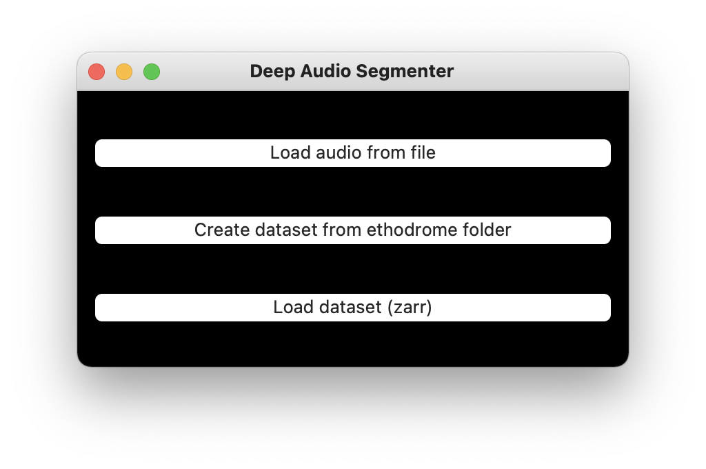
Start screen.#
Load audio data#
Choose Load audio from file and select the downloaded recording of fly song.
In the dialog that opens, leave everything as is except set Minimal/Maximal spectrogram frequency—the range of frequencies in the spectrogram display—to 50 and 1000 Hz. This will restrict the spectrogram view to only show the frequencies found in fly song.
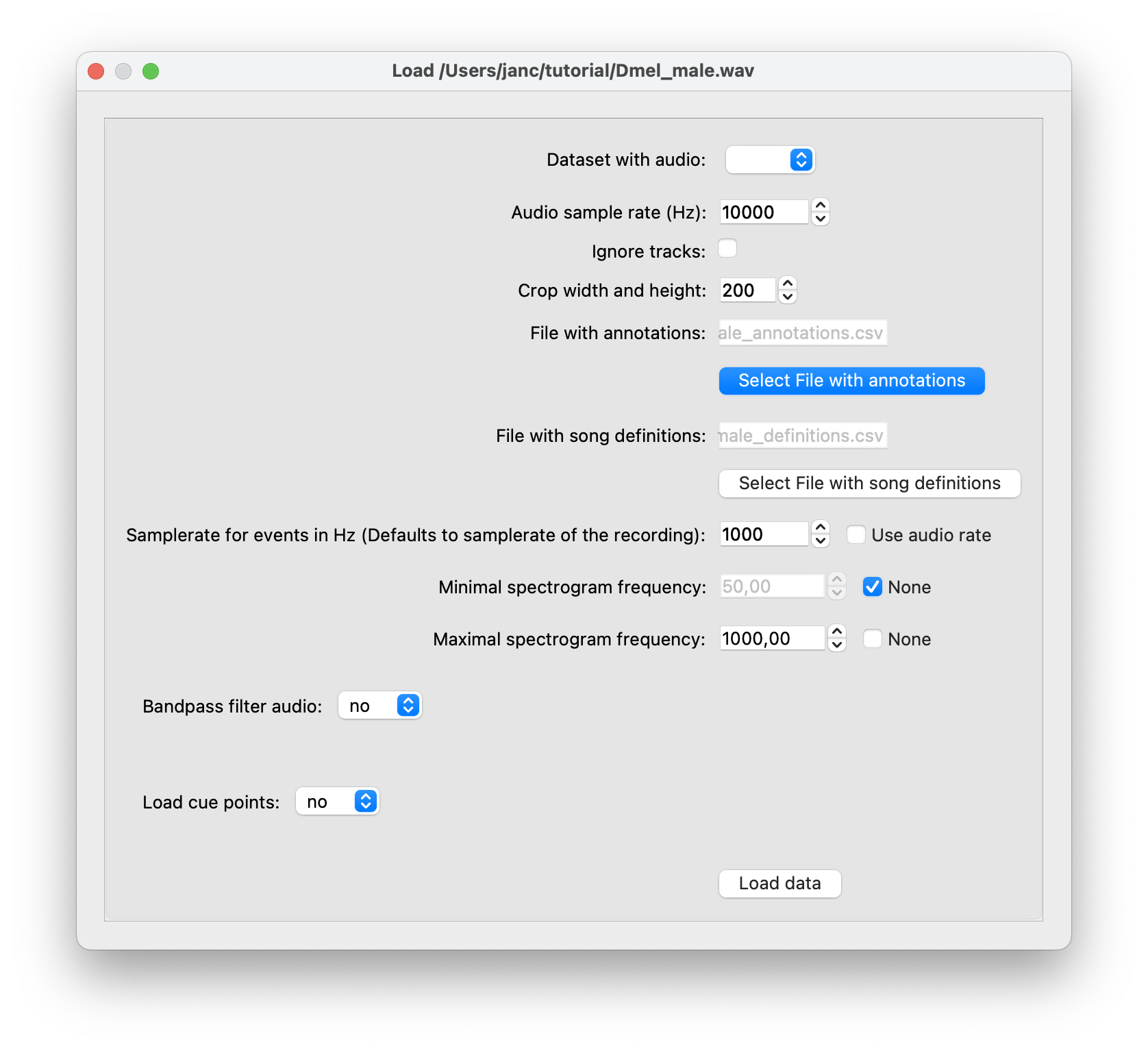
Loading screen.#
Waveform and spectrogram display#
Loading the audio will open a window that displays the first second of audio as a waveform (top) and a spectrogram (bottom). You will see the two major modes of fly song—pulse and sine. The recording starts with sine song—a relatively soft oscillation resulting in a spectral power at ~150 Hz. Pulse song starts after ~0.75 seconds, evident as trains of brief wavelets with a regular interval.
To navigate the view: Move forward/backward along the time axis via the A/D keys and zoom in/out the time axis with the W/S keys (see also the Playback menu). You can also navigate using the scroll bar below the spectrogram display or jump to specific time points using the text field to the right of the scroll bar. The temporal and frequency resolution of the spectrogram can be adjusted with the R and T keys.
You can play back the waveform on display through your headphones/speakers by pressing E.
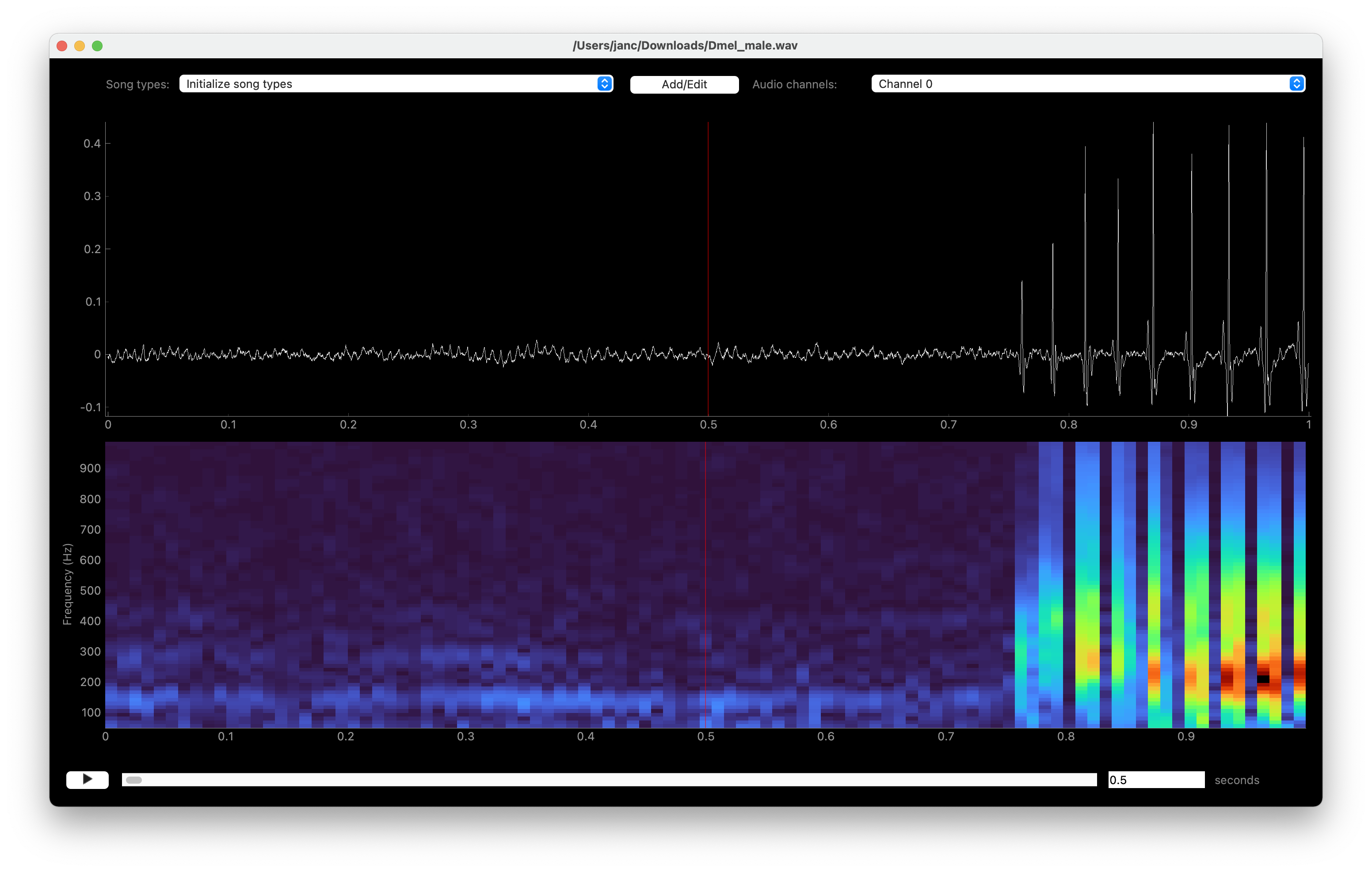
Waveform (top) and spectrogram (bottom) display of fly song.#
Initialize or edit song types#
Before you can annotate song, you need to register the sine and pulse song types for annotation. DAS discriminates two principal categories of song types:
Segments are song types that extend over time and are defined by a start and a stop time. The aforementioned sine song and the syllables of mouse and bird vocalizations fall into the segment category.
Events are defined by a single time of occurrence. The aforementioned pulse song is a song type of the event category.
Add two new song types for annotation via the Add/edit button at the top of the windows or via the Annotations/Add or edit song types menu: ‘pulse’ of category ‘event’ and ‘sine’ of category ‘segment’:
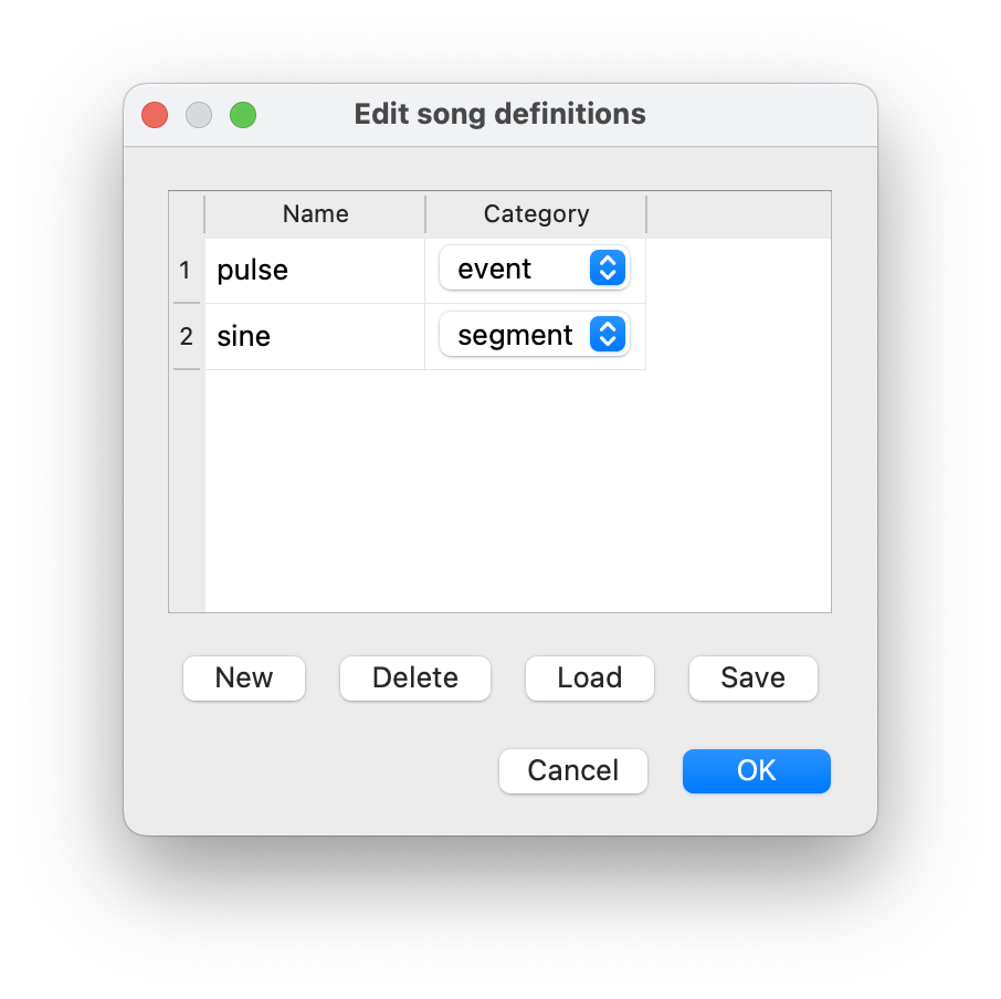
Create two new song types for annotation.#
Create annotations manually#
The two new song types pulse or sine can now be activated for annotation using the dropdown menu on the top left of the window. The active song type can also be changed with the number keys indicated in the dropdown menu—in this case 1 activates pulse, 2 activates sine.
Song is annotated by left-clicking the waveform or spectrogram view. If an event-like song type is active, a single left click marks the time of an event. A segment-like song type requires two clicks—one for each boundary of the segment.
Left clicks in waveform or spectrogram view create annotations.#
Annotate by thresholding the waveform#
Annotation of events can be sped up with a “Thresholding mode”, which detects peaks in the sound energy exceeding a threshold. Activate thresholding mode via the Annotations menu. This will display a draggable horizontal line—the detection threshold—and a smooth pink waveform—the envelope of the waveform. Adjust the threshold so that only “correct” peaks in the envelope cross the threshold and then press I to annotate these peaks as events.
Annotations assisted by thresholding and peak detection.#
Edit annotations#
In case you misclicked, you can edit and delete annotations. Edit event times and segment bounds by dragging the lines or the boundaries of segments. Drag the shaded area itself to move a segment without changing its duration. Movement can be disabled completely or restricted to the currently selected annotation type via the Annotations menu.
Delete annotations of the active song type by right-clicking on the annotation. Annotations of all song types or of only the active one in the view can be deleted with U and Y, respectively, or via the Annotations menu.
Dragging moves, right click deletes annotations.#
Change the label of an annotation via CMD/CTRL+Left click on an existing annotation. The type of the annotation will change to the currently active one.
Export annotations and make a dataset#
DAS achieves good performance from few annotated examples. Once you have completely annotated the song in the first 18 seconds of the tutorial recording—all pulses and sine song segments in that section of the song—you can train a network to help with annotating the rest of the data.
Training requires the audio data and the to be in a specific format. First, export the audio data and the annotations via File/Export for DAS to a new folder (not the one containing the original audio)—let’s call the folder quickstart. In the following dialog set start seconds and end seconds to the annotated time range: 0 and 18 seconds, respectively.
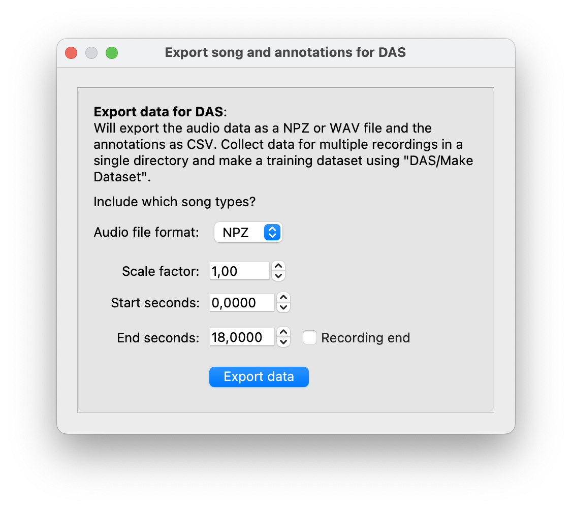
Export audio data and annotations for the annotated range from 0 to 18 seconds.#
Then make a dataset, via DAS/Make dataset for training. In the file dialog, select the quickstart folder you exported your annotations into. In the next dialog, we will adjust how data is split into training, validation and testing data. For the small data set annotated in the first step of this tutorial, we will not test the model, to maximize the data available for optimizing the network (training and validation). Set the training split to 0.60, the validation split to 0.40 and the test split to 0.00 (not test):
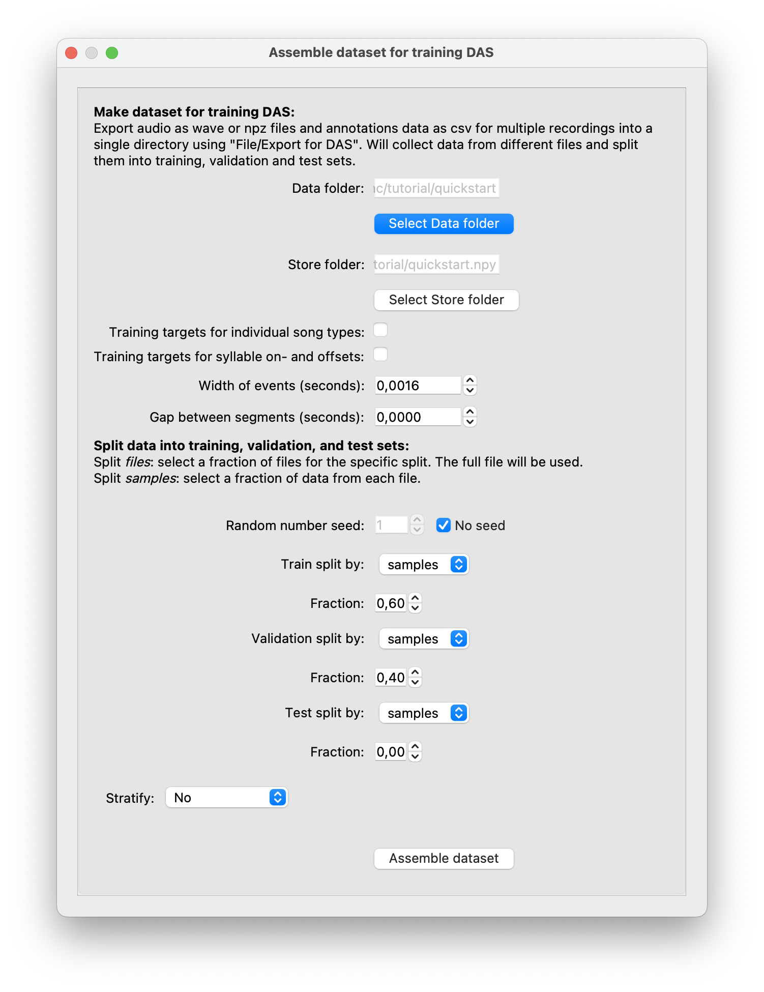
Make a dataset for training.#
This will create a dataset folder called quickstart.npy that contains the audio data and the annotations formatted for training.
Fast training#
Configure a network and start training via DAS/Train. This will ask you to select folder with the dataset you just created, quickstart.npy. Then, a dialog allows you to configure the network. For the fast training change the following:
Set
Downsampling frontendtoNone.Set both
Number of filtersandFilter duration (samples)to 16. This will result in a smaller network with fewer parameters, which will train faster.Set
Number of epochsto 10, to finish training earlier.
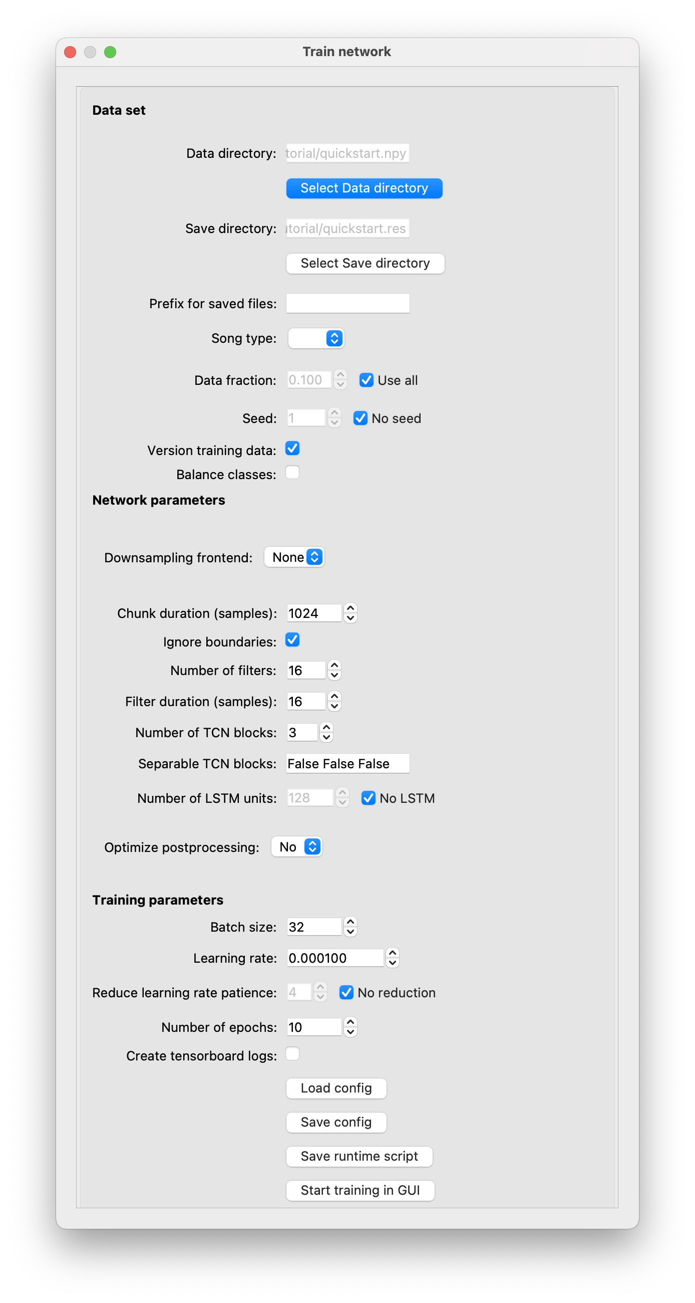
Train options#
Then hit Start training in GUI—this will start training in a background process. A small window will display training progress (see also the output in the terminal). Training with this small dataset will finish in 10 minutes on a CPU and in 2 minutes on a GPU. For larger datasets, we highly recommend training on a machine with a discrete Nvidia GPU.
Predict#
Once training finished, generate annotations using the trained network via DAS/Predict. This will ask you to select a model file containing the trained model. Training creates files in the quickstart.res folder, starting with the time stamp of training—select the file ending in _model.h5.
In the next dialog, predict song for 60 seconds starting after your manual annotations:
Set
Start secondsto 18 andEnd secondsto 78.Make sure that
Proof reading modeis enabled. That way, annotations created by the network will be assigned names ending in_proposals- in our casesine_proposalsandpulse_proposals. The proposals will be transformed into propersineandpulseannotations during proof reading.Enable
Fill gaps shorter than (seconds)andDelete segments shorter than (seconds)by unchecking both check boxes.
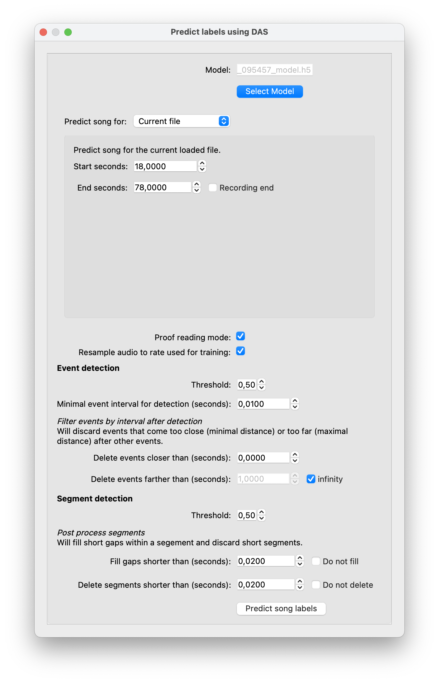
Predict annotations for the next 60 seconds of audio.#
In contrast to training, prediction is very fast, and does not require a GPU—it should finish after 30 seconds. The proposed annotations should be already good. Most pulses should be correctly detected. Sine song is harder to predict and may be often or chopped up into multiple segments with gaps in between.
Proof reading#
To turn the proposals into proper annotations, fix and approve them. Correct any prediction errors—add missing annotations, remove false positive annotations, adjust the timing of annotations. See Create annotations and Edit annotations. Once you have corrected all errors in the view, select the proposals type you want to fix (sine_proposals or pulse_proposals), and approve the corresponding annotations with G. This will rename the proposals in the view to the original names (for instance, sine_proposals -> sine). Alternatively, H will approve proposals of all song types in view.
Go back to “Export”#
Once all proposals have been approved, export all annotations (now between 0 and 78 seconds), make a new dataset, train, predict, and repeat. Every prediction should use the latest model in the quickstart.res folder. If prediction performance is adequate, fully train the network by increasing the Number of epochs to a larger number (400, for example), and this time using a completely new recording as the test set. Alternatively, you can use the same recording and split by samples.
Once the model is good enough to predict on new recordings, uncheck Proof reading mode on these recordings so the annotations produced have the proper ‘pulse’ and ‘sine’ labels.