Quick start tutorial (bird)

This quick start tutorial walks through all steps required to make DAS work with your data, using recordings of zebra finch song as an example. A comprehensive description of all menus and options is available in the GUI documentation.

We will use an iterative annotation workflow: annotate a few song motifs, fast-train a network on those annotations, and use that network to propose annotations for a second recording. Correcting proposals is typically much faster than annotating everything from scratch. Repeat this annotate-train-predict cycle with progressively larger datasets until performance is satisfactory.

Download example data

Download these two audio files from this tutorial:

• birdname_130519_110831.1.wav — training recording

• birdname_130519_113526.55.wav — test recording

The recordings are of a male zebra finch, recorded by Jack Goffinet et al. as part of this dataset.

Start the GUI

Install the PyPI version of DAS following the installation instructions. Then open a terminal, activate the conda environment created during installation, and start the GUI:

conda activate das
das gui

The following window should open:

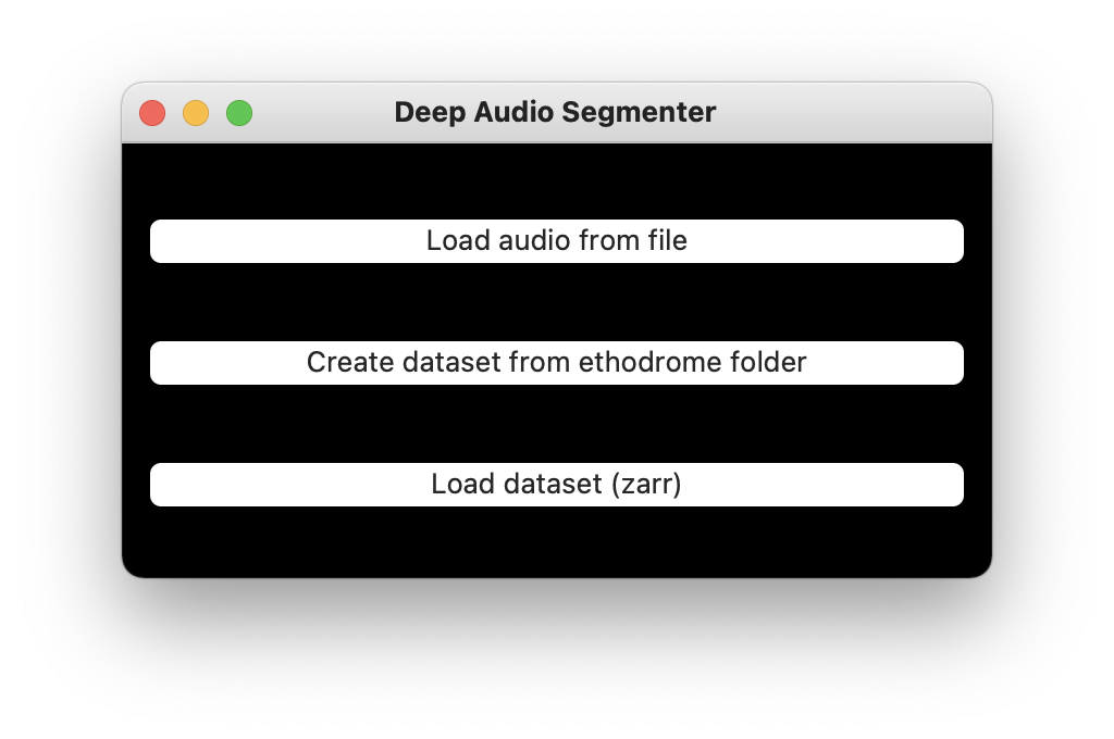
Start screen.

Load audio data

Choose Load audio from file and select the training recording, birdname_130519_110831.1.wav.

In the dialog that opens, leave the automatically detected audio sample rate unchanged. Leave the annotation and song-definition fields at their defaults, select Use audio rate, and load the data.

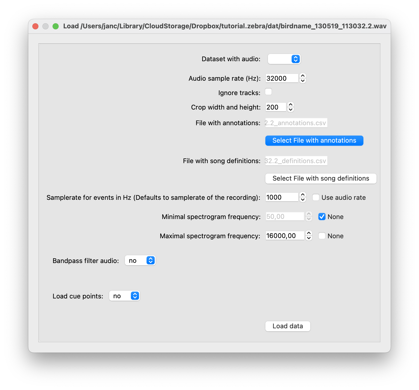
Loading the training recording.

Waveform and spectrogram display

Loading the audio opens a window that displays the waveform (top) and spectrogram (bottom).

Move forward or backward with D or A, and zoom in or out with W or S (see also the Playback menu). You can also navigate with the scroll bar below the spectrogram or jump to a time using the field to its right. Adjust the temporal and frequency resolution of the spectrogram with R and T.

Play the displayed audio through your headphones or speakers by pressing E.

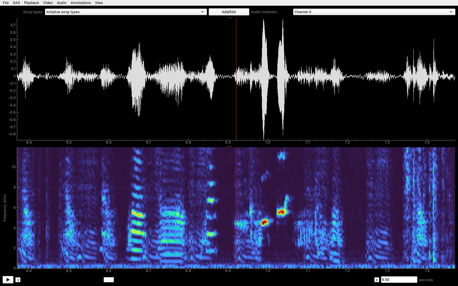
Waveform (top) and spectrogram (bottom) of zebra finch song.

Initialize syllable types

Before annotating, register the six syllable types in this bird’s motif. Open the editor with the Add/Edit button above the plots or via Annotations/Add or edit song types, and create six segment types named syll1 through syll6.

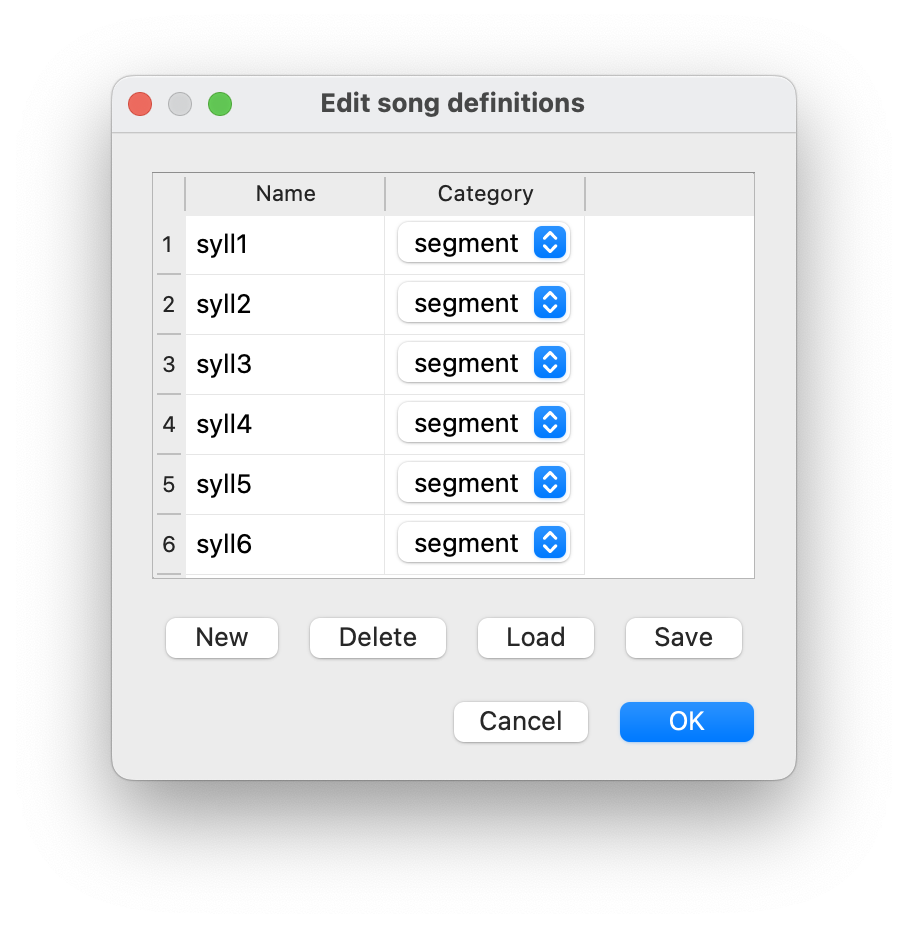
Create six syllable types for annotation.

Create annotations manually

Select a syllable type from the menu above the plots. You can also switch types with the number keys shown in that menu—in this case 1 through 6.

Annotate a syllable by left-clicking the waveform or spectrogram twice: once at the onset and once at the offset.

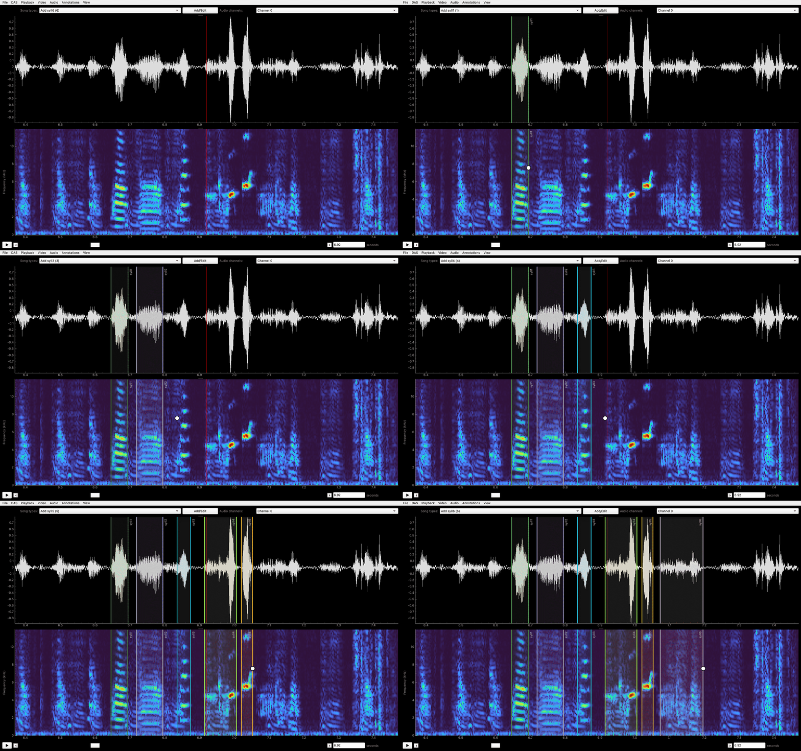
Left-click at each syllable’s onset and offset to create annotations.

Edit annotations

Correct a syllable boundary by dragging it. Drag the shaded segment itself to move the syllable without changing its duration. Movement can be disabled or restricted to the selected syllable type in the Annotations menu.

Delete an annotation with a right-click. You can also delete all annotations in view with U, or only annotations of the selected type with Y. Change an annotation’s label by selecting the desired type and using CMD/CTRL+left-click on the annotation.

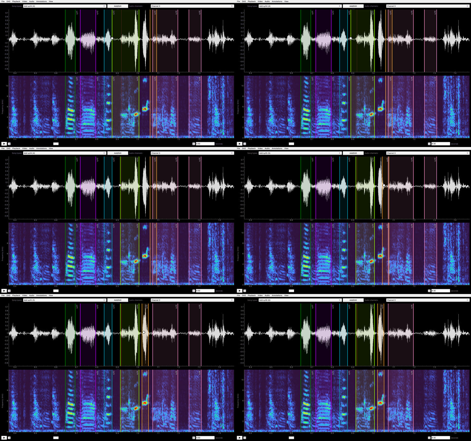
Drag to correct boundaries or move segments; right-click to delete.

Export annotations and make a dataset

Once you have annotated the six syllables in all 14 motifs of the training recording, you can train a network to help annotate more data.

Training requires audio and annotations in a specific format. Export them via File/Export for DAS to a new folder—not the folder containing the original audio. Name the new folder quickstart.

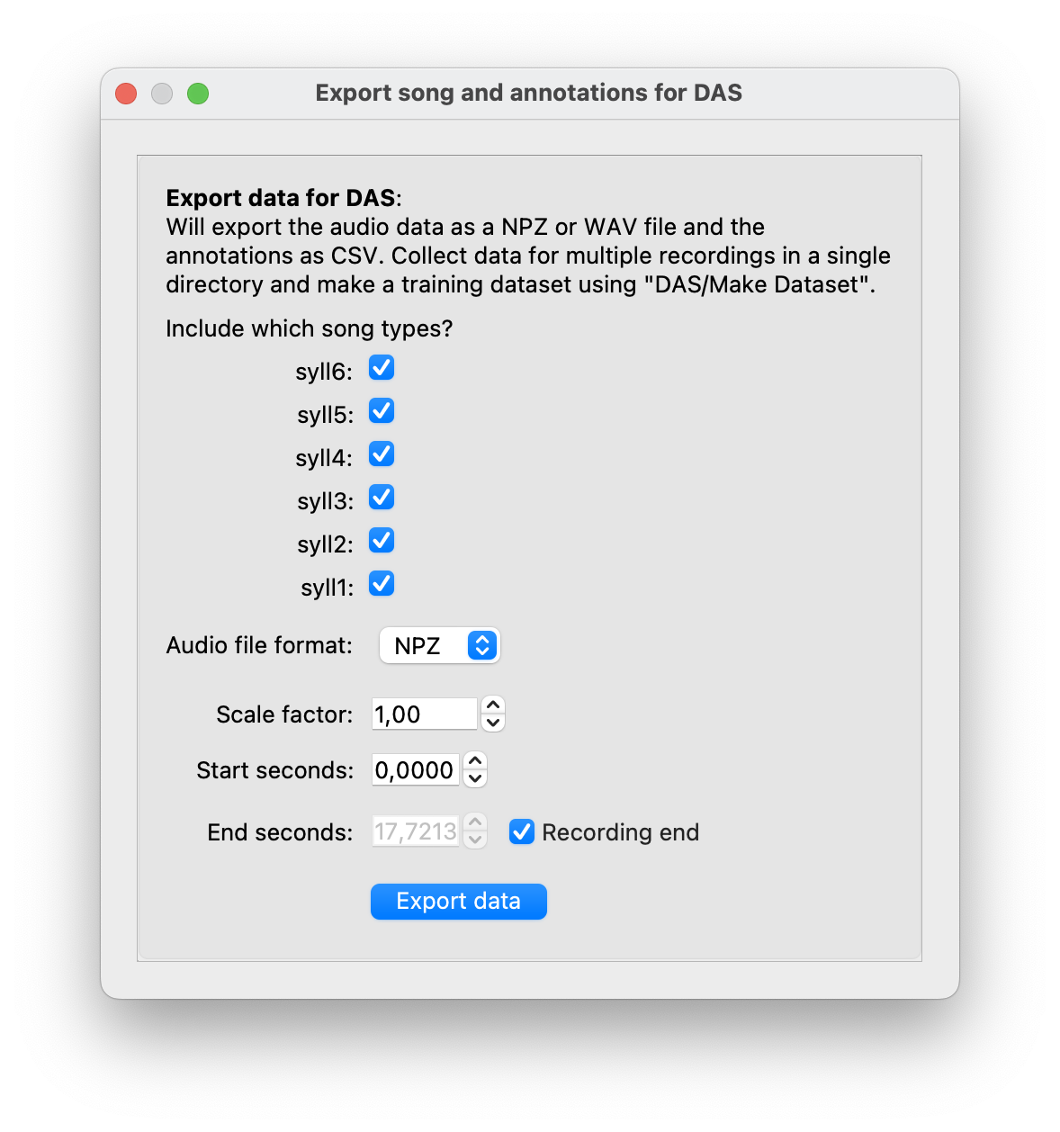
Export audio and annotations for the complete recording.

Next, choose DAS/Make dataset for training and select the quickstart folder. For this small initial dataset, use the annotations for training and validation only: set the training split to 0.60, validation split to 0.40, and test split to 0.0.

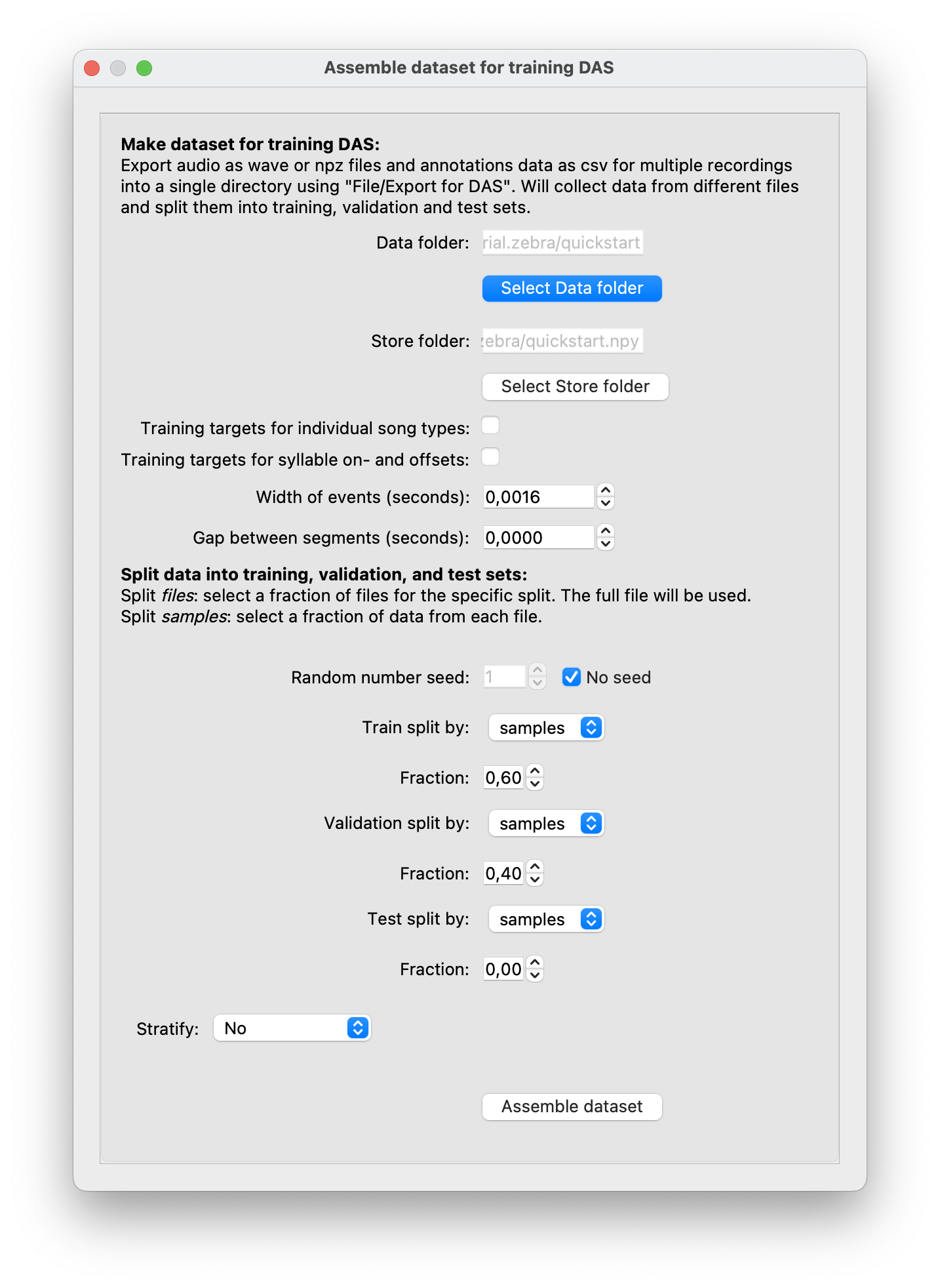
Make a dataset for training.

This creates a dataset named quickstart.npy containing the audio and annotations in the format required for training.

Fast training

Choose DAS/Train, select the quickstart.npy dataset, and configure the network. For this fast training run, change:

• Chunk duration (samples) to 4096

• Number of filters to 64

• Filter duration (samples) to 32

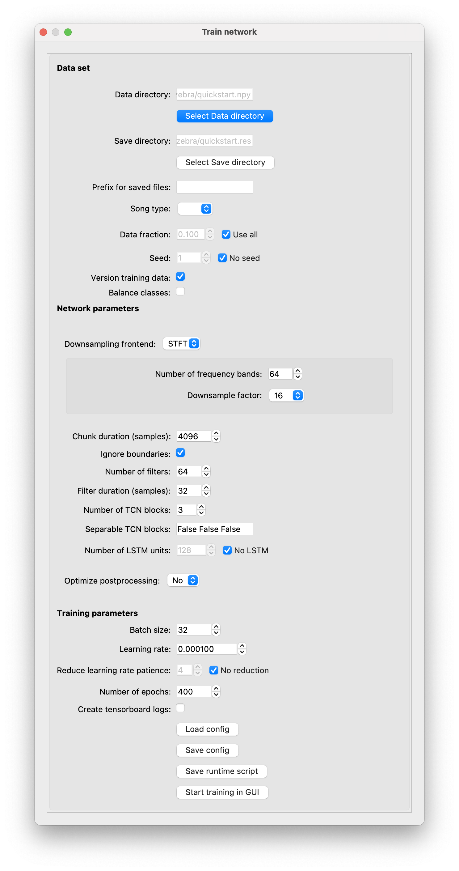
Training options.

Select Start training in GUI. Training runs in a background process, and a small window and the terminal show its progress. Runtime depends strongly on your computer; a GPU is recommended for larger datasets.

Predict

When training finishes, load the test recording, birdname_130519_113526.55.wav. Choose DAS/Predict, select the trained model in the quickstart.res folder, and choose the file ending in _model.keras.

In the prediction dialog:

• Leave Start seconds at 0 and Recording end selected to predict the complete test recording.

• Keep Proof reading mode enabled. Predictions will be named syll1_proposals through syll6_proposals until you approve them.

• Enable Fill gaps shorter than (seconds) by clearing Do not fill, and set the value to 0.005.

• Enable Delete segments shorter than (seconds) by clearing Do not delete, and leave the value at 0.020.

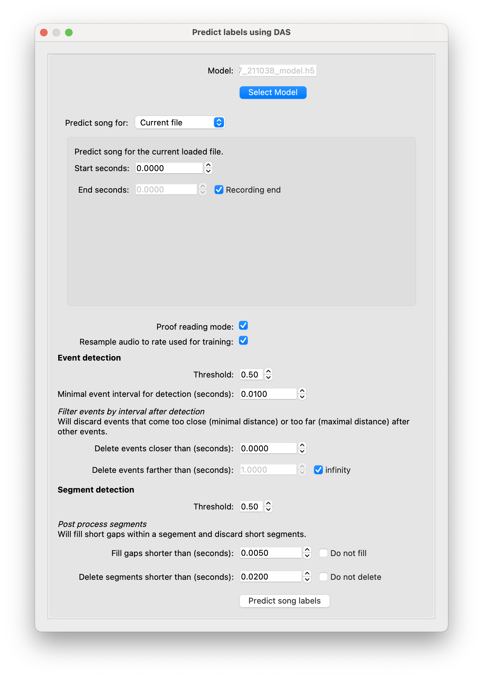
Predict annotations for the complete test recording.

Prediction is much faster than training and does not require a GPU. Most proposed syllables should be detected correctly, but there may be false positives, missed or confused syllables, and imprecise boundaries.

Proofread

Correct the proposals: add missed syllables, delete false positives, fix label errors, and adjust syllable boundaries using the annotation tools described above. Once all proposals in view are correct, approve them with H.

Repeat from export

Export the approved annotations for this recording into the same quickstart folder. Make a new dataset, train again, predict more data, and repeat. When prediction performance is adequate, fully train the network with a separate recording reserved as a test set and with more training epochs.