Descriptive statistics#
So far we encountered the mean and the standard deviation as descriptive statistics. These two quantities are sufficient to fully describe normally distributed data! Alas, not all data is normally distributed so we need other measures of central tendency and dispersion.
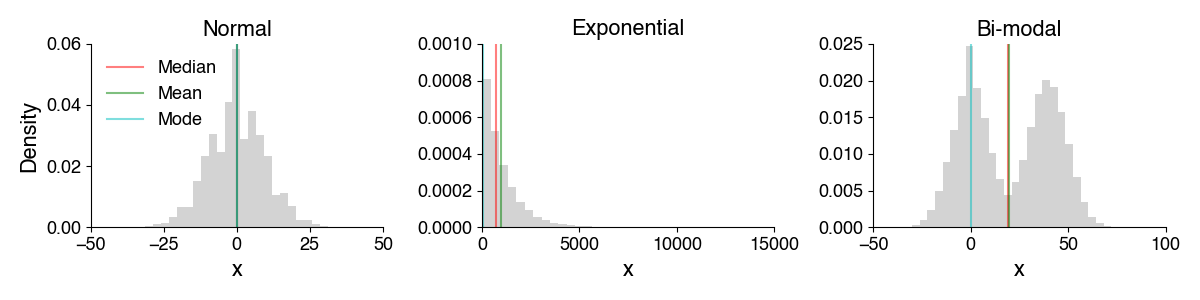
Measures of central tendency: Mean, median, mode#
Mean: Average value: \(1/N \sum_i^N x_i\)
Median: Value at the midpoint of the distribution, such that there is an equal probability of observing values below and above the median (50% of the samples are below the median, 50% above).
Mode: Most frequent value for a discrete distribution or the point at which a continuous pdf (histogram) attains its max value.
For a normal distribution, mean, median, and mode are identical.
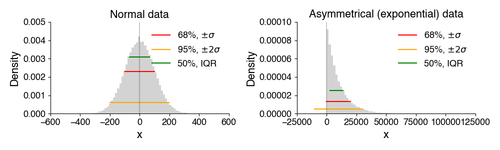
Measures of dispersion: Variance, standard deviation and inter-quartile range#
Variance: \(\sigma^2 = 1/(N-1) \sum_i^N (x_i - \hat{x})^2\) (\(\hat{x}\) is the mean of all x)
Standard deviation is the square root of the variance: \(\sigma = \sqrt{\sigma^2}\). Useful for normal data.
Inter-quartile range (IQR): Quartiles split the data into 4 parts each with equal number of samples - the first quartile contains the 25% of samples with the lowest values, the last quartile contains the 25% of the samples with the highest values. The interquartile range is the range of data that spans the central 50% of the distribution. Useful for non-normal (asymmetrical) data.
Note The variance measures the average squared distance of the samples from the sample mean. Why then use a normalizaton factor of \(N-1\), instead of \(N\) as expected for an average? Turns out the values obtained with normalization \(N\) are biased - you will explore this in the exercise.
Mini Exercise#
Visualize the density distribution of the data in x
Calculate and plot the mean and the median of the distribution as vertical lines. Why is the mean greater than the median?
import numpy as np
import matplotlib.pyplot as plt

x = np.random.weibull(.4, (1_000_000))  # generate 1M random numbers from a probability distribution

# your solution here
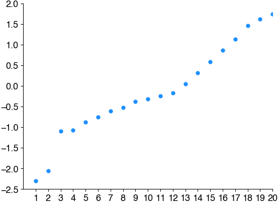
Percentiles#
Median and quartiles are special cases of percentiles. A percentile is the value at or below which a given percentage of all samples falls.
The median is the 50th percentile - 50% of all samples fall below the median.
The first quartile is the 25th percentile - 25% (a quarter) of all samples fall below the quartile.
99% of all samples fall below the 99th percentile.
np.random.seed(1)
y = np.random.randn(20)  # generate 20 random numbers

y.sort()  # sort them
rank = np.arange(1, len(x)+1)  # the rank is the position of a value when the data is sorted from lowest to highest, like a ranking in sports.
print(np.around(y, decimals=2))

plt.plot(rank, y, 'o', c='dodgerblue')
plt.xticks(rank)
plt.show()

# Where is the median?
# Where is the first quartile?
# Where is the 10th perentile?
# Where is the 90th perentile?
# Where is the 99th perentile?
[-2.3  -2.06 -1.1  -1.07 -0.88 -0.76 -0.61 -0.53 -0.38 -0.32 -0.25 -0.17
  0.04  0.32  0.58  0.87  1.13  1.46  1.62  1.74]