Working with tabular data: Pandas#
Pandas provides three things:
a new data type specifically designed for tabular data - the
DataFramefunctions for manipulating tabular data
IO for tabular data (covered in Week3/Files)
Why yet another data type?#
Numpy arrays can hold tabular data - 2D matrices. So why do we need another, special data type? One problem with raw 2D arrays is that they are not self-documenting. What does that mean?
Take the data from exercise of Week3/Files: We calculated behavioral scores, stored them in a numpy array, and saved the array to a text file:
import numpy as np
# load and print matrix
scores = np.loadtxt('dat/pd_scores.txt')
scores
array([[0.08656877, 0.26186048],
       [0.27081788, 0.48948194],
       [0.47072199, 0.65700287],
       [0.55996639, 0.81680243],
       [0.84880959, 0.98686545],
       [0.91045131, 0.99465925]])
Do you remember what the data means? What are the individual rows? What are the columns? Imagine this were an analysis on your own data and you’d want to look at the results in 3 months or so.
There are no labels, so it’s hard to know from the data itself what they mean - the data is not “self-documenting”
We can turn this into a DataFrame:
import pandas as pd

# the folder names correspond to the days
days = ['20230912','20230913','20230914','20230915','20230916','20230917']

# make DataFrame - no need to understand the specifics - I will explain soon what is going on here
# we can easily turn a dictionary into a DataFrame - keys will be column labels, values are the per-row data
# we can also specify row labels - an index.
scores_dict = {'intial score': scores[:, 0], 'final score': scores[:, 1]}
df = pd.DataFrame(scores_dict, index=days)
df
| intial score | final score | |
|---|---|---|
| 20230912 | 0.086569 | 0.261860 |
| 20230913 | 0.270818 | 0.489482 |
| 20230914 | 0.470722 | 0.657003 |
| 20230915 | 0.559966 | 0.816802 |
| 20230916 | 0.848810 | 0.986865 |
| 20230917 | 0.910451 | 0.994659 |
You can save the data frame as csv and excel, and reload them as a DataFrame, with the labels being preserved:
df.to_csv('dat/scores_df.csv')
df.to_excel('dat/scores_df.xlsx')

# load data
df_from_file = pd.read_csv('dat/scores_df.csv', index_col=0, )
df_from_file
| Unnamed: 0 | final score | |
|---|---|---|
| intial score | ||
| 0.086569 | 20230912 | 0.261860 |
| 0.270818 | 20230913 | 0.489482 |
| 0.470722 | 20230914 | 0.657003 |
| 0.559966 | 20230915 | 0.816802 |
| 0.848810 | 20230916 | 0.986865 |
| 0.910451 | 20230917 | 0.994659 |
Creating DataFrames#
We already learned that pandas provides versatile file I/O (csv, excel): https://pandas.pydata.org/docs/_sources/user_guide/io.html (see Week3/Files)
As shown above, a DataFrame can be created from Dictionary.
Data is 2D and is organized in columns and rows (rows=index). If we do not specify an index during DataFrame creation, it will be generated automatically, as a row numbers:
d = {'column 1': ['a','b','c'], 'column 2': [10, 20, 30]}

print(d)
df = pd.DataFrame(d)
df
{'column 1': ['a', 'b', 'c'], 'column 2': [10, 20, 30]}
| column 1 | column 2 | |
|---|---|---|
| 0 | a | 10 |
| 1 | b | 20 |
| 2 | c | 30 |
A DataFrame can also be created from a 2D np.array. In that case, we can specify the column names separately:
# scores
days
['20230912', '20230913', '20230914', '20230915', '20230916', '20230917']
df = pd.DataFrame(scores, columns=['initial', 'final'], index=days)
df
| initial | final | |
|---|---|---|
| 20230912 | 0.086569 | 0.261860 |
| 20230913 | 0.270818 | 0.489482 |
| 20230914 | 0.470722 | 0.657003 |
| 20230915 | 0.559966 | 0.816802 |
| 20230916 | 0.848810 | 0.986865 |
| 20230917 | 0.910451 | 0.994659 |
Accessing data in DataFrames#
There are many ways of accessing data in a DataFrame. We cover the basics here.
More details: https://pandas.pydata.org/docs/_sources/user_guide/indexing.html
Access columns like a dictionary#
df['final'] # df[column_name]
20230912    0.261860
20230913    0.489482
20230914    0.657003
20230915    0.816802
20230916    0.986865
20230917    0.994659
Name: final, dtype: float64
Access rows and columns by name like a 2D dictionary via df.loc#
df.loc[index_name, column_name]
df = pd.DataFrame(scores, columns=['initial', 'final'], index=days)
display(df)

df.loc[:, 'initial']


# print("by row name - all columns: df.loc['20230915']")
# print(df.loc['20230915'])

# print("this is equivalent to: df.loc['20230915', :]")
# print(df.loc['20230915', :])

# print("by column name - all rows, one column: df.loc[:, 'initial']")
# print(df.loc[:, 'initial'])

# print("\nby row and column name - returns a single cell in the table: df.loc['20230915', 'initial']")
# print(df.loc['20230915', 'initial'])
| initial | final | |
|---|---|---|
| 20230912 | 0.086569 | 0.261860 |
| 20230913 | 0.270818 | 0.489482 |
| 20230914 | 0.470722 | 0.657003 |
| 20230915 | 0.559966 | 0.816802 |
| 20230916 | 0.848810 | 0.986865 |
| 20230917 | 0.910451 | 0.994659 |
20230912    0.086569
20230913    0.270818
20230914    0.470722
20230915    0.559966
20230916    0.848810
20230917    0.910451
Name: initial, dtype: float64
Access to rows and columns via a numerical index like a 2D array via df.iloc#
df.iloc[row_number, column_number]
print(df.iloc[:, 1])
print(df.iloc[1])
print(df.iloc[1, :])
print(df.iloc[2, 1])
print(df.iloc[:2, 1])  # slicing also works
20230912    0.261860
20230913    0.489482
20230914    0.657003
20230915    0.816802
20230916    0.986865
20230917    0.994659
Name: final, dtype: float64
initial    0.270818
final      0.489482
Name: 20230913, dtype: float64
initial    0.270818
final      0.489482
Name: 20230913, dtype: float64
0.6570028706902653
20230912    0.261860
20230913    0.489482
Name: final, dtype: float64
Mini-Exercise:#
Get from the DataFrame below:
all data from the ‘test’ column
all data from the ‘…’ row
data from the cell at row ‘…’ and column ‘…’
the data from the 5th row
df = pd.DataFrame(...)
Access the underlying data like a numpy array:#
data = df.values
data, type(data)
(array([[0.08656877, 0.26186048],
        [0.27081788, 0.48948194],
        [0.47072199, 0.65700287],
        [0.55996639, 0.81680243],
        [0.84880959, 0.98686545],
        [0.91045131, 0.99465925]]),
 numpy.ndarray)
Boolean indexing also works#
df[df['initial'] < 0.4]
| initial | final | |
|---|---|---|
| 20230912 | 0.086569 | 0.261860 |
| 20230913 | 0.270818 | 0.489482 |
You can apply boolean indices repeatedly, to filter by different conditions:
df = pd.DataFrame({'name': ['Tim', 'Jim', 'Pim', 'Pip', 'Tom'],
                   'age': [12, 24, 18, 22, 26],
                   'score': [4, 0, 8, 9, 7]})
display(df)

# first, keep only the old one - age>20 yrs
old_guys = df[df['age']> 20]
display(old_guys)

# then, filter the dataframe with the old ones, to keep only the high scores - score>4
high_scorer = old_guys[old_guys['score']> 4]
display(high_scorer)
| name | age | score | |
|---|---|---|---|
| 0 | Tim | 12 | 4 |
| 1 | Jim | 24 | 0 |
| 2 | Pim | 18 | 8 |
| 3 | Pip | 22 | 9 |
| 4 | Tom | 26 | 7 |
| name | age | score | |
|---|---|---|---|
| 1 | Jim | 24 | 0 |
| 3 | Pip | 22 | 9 |
| 4 | Tom | 26 | 7 |
| name | age | score | |
|---|---|---|---|
| 3 | Pip | 22 | 9 |
| 4 | Tom | 26 | 7 |
Groupby: Split-apply-combine#
A common problem in data analysis is:
We have an experiment with multiple subjects, and multiple measurements per subject. We’d like to compute the average score for each subject for plotting and statistics.
For instance:
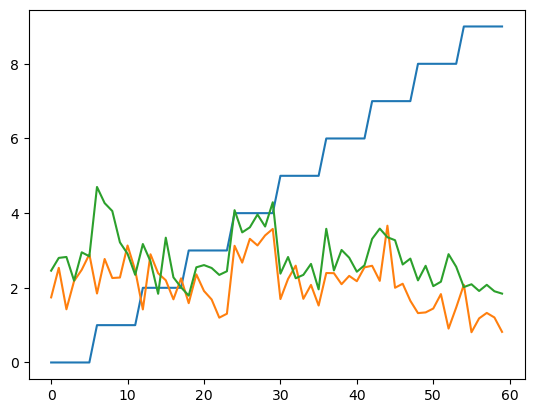
# REMOVE - make dummy data for grouped stats
import matplotlib.pyplot as plt
nb_animals = 10
nb_trials = 6

scores = np.zeros((nb_animals * nb_trials, 3))
for ani, animal in enumerate(range(nb_animals)):
    scores[(ani) * nb_trials:(ani + 1) * nb_trials, 1:] = 2+np.random.randn(nb_trials, 2)/2 + np.array([0.3, 0.8]) + np.random.randn(1) / 2
    scores[(ani) * nb_trials:(ani + 1) * nb_trials, 0] = animal

plt.plot(scores)

df = pd.DataFrame({'animal': scores[:, 0], 'pre': scores[:,1], 'post': scores[:,2]})
df.to_csv('dat/groupby.csv', index=None)
df = pd.read_csv('dat/pd_groupby.csv')
df
| animal | pre | post | |
|---|---|---|---|
| 0 | 0.0 | 2.211986 | 3.107796 |
| 1 | 0.0 | 2.204871 | 2.830730 |
| 2 | 0.0 | 2.560633 | 3.483980 |
| 3 | 0.0 | 1.476412 | 2.801709 |
| 4 | 0.0 | 3.662519 | 3.447005 |
| 5 | 0.0 | 2.538696 | 3.301515 |
| 6 | 1.0 | 1.867229 | 3.484270 |
| 7 | 1.0 | 3.306150 | 3.077195 |
| 8 | 1.0 | 2.741388 | 2.586878 |
| 9 | 1.0 | 1.874149 | 3.264328 |
| 10 | 1.0 | 3.276006 | 2.503612 |
| 11 | 1.0 | 3.363795 | 3.175878 |
| 12 | 2.0 | 3.645122 | 3.871356 |
| 13 | 2.0 | 4.419345 | 3.223414 |
| 14 | 2.0 | 3.157167 | 2.851897 |
| 15 | 2.0 | 3.075222 | 3.591049 |
| 16 | 2.0 | 3.085689 | 4.618074 |
| 17 | 2.0 | 2.799818 | 3.586372 |
| 18 | 3.0 | 2.717420 | 3.483265 |
| 19 | 3.0 | 1.267145 | 2.402146 |
| 20 | 3.0 | 3.497071 | 2.818079 |
| 21 | 3.0 | 1.207408 | 2.662157 |
| 22 | 3.0 | 2.392043 | 2.872839 |
| 23 | 3.0 | 2.845028 | 2.683747 |
| 24 | 4.0 | 1.963877 | 1.633267 |
| 25 | 4.0 | 2.557404 | 1.549594 |
| 26 | 4.0 | 1.115516 | 2.964476 |
| 27 | 4.0 | 1.830395 | 1.952609 |
| 28 | 4.0 | 2.170095 | 2.525734 |
| 29 | 4.0 | 2.586667 | 2.240448 |
| 30 | 5.0 | 2.045121 | 3.573011 |
| 31 | 5.0 | 2.054961 | 3.010360 |
| 32 | 5.0 | 2.021420 | 3.538843 |
| 33 | 5.0 | 1.626790 | 2.702867 |
| 34 | 5.0 | 2.342304 | 2.389883 |
| 35 | 5.0 | 1.800452 | 3.311980 |
| 36 | 6.0 | 0.641648 | 1.322786 |
| 37 | 6.0 | 2.275206 | 0.707293 |
| 38 | 6.0 | 1.090543 | 1.291870 |
| 39 | 6.0 | 1.289345 | 1.976258 |
| 40 | 6.0 | 1.828772 | 1.341221 |
| 41 | 6.0 | 0.982321 | 2.676962 |
| 42 | 7.0 | 3.179301 | 4.185368 |
| 43 | 7.0 | 3.756986 | 3.681570 |
| 44 | 7.0 | 2.070850 | 3.249996 |
| 45 | 7.0 | 2.405634 | 3.025023 |
| 46 | 7.0 | 3.773297 | 3.787543 |
| 47 | 7.0 | 3.351603 | 3.171412 |
| 48 | 8.0 | 2.075409 | 3.820043 |
| 49 | 8.0 | 1.989337 | 2.970652 |
| 50 | 8.0 | 2.469318 | 2.046087 |
| 51 | 8.0 | 2.054879 | 2.514335 |
| 52 | 8.0 | 1.448087 | 2.380560 |
| 53 | 8.0 | 2.552318 | 3.016450 |
| 54 | 9.0 | 2.369584 | 1.889417 |
| 55 | 9.0 | 3.086123 | 2.560759 |
| 56 | 9.0 | 2.097187 | 2.446292 |
| 57 | 9.0 | 1.857415 | 0.800996 |
| 58 | 9.0 | 1.498517 | 1.811201 |
| 59 | 9.0 | 0.719002 | 2.691326 |
We can solve this using for loops and boolean indexing:
# identify all animals
animals = df['animal'].unique()

# example of boolean indexing
display(df[df['animal']==0.0])
# compute the mean:
display(df[df['animal']==0.0].mean())
display(np.mean(df[df['animal']==0.0], axis=0))

# loop over all animals
animal_avg = []
for animal in animals:
    animal_avg.append(df[df['animal']==animal].mean().values)
animal_avg
| animal | pre | post | |
|---|---|---|---|
| 0 | 0.0 | 2.211986 | 3.107796 |
| 1 | 0.0 | 2.204871 | 2.830730 |
| 2 | 0.0 | 2.560633 | 3.483980 |
| 3 | 0.0 | 1.476412 | 2.801709 |
| 4 | 0.0 | 3.662519 | 3.447005 |
| 5 | 0.0 | 2.538696 | 3.301515 |
animal    0.000000
pre       2.442519
post      3.162122
dtype: float64
animal    0.000000
pre       2.442519
post      3.162122
dtype: float64
[array([0.        , 2.44251943, 3.16212242]),
 array([1.        , 2.73811958, 3.01536034]),
 array([2.        , 3.36372726, 3.62369364]),
 array([3.        , 2.32101921, 2.82037202]),
 array([4.        , 2.03732544, 2.14435453]),
 array([5.        , 1.98184125, 3.0878241 ]),
 array([6.        , 1.35130571, 1.55273191]),
 array([7.        , 3.08961177, 3.51681884]),
 array([8.        , 2.09822498, 2.79135462]),
 array([9.        , 1.9379714 , 2.03333186])]
This series of steps is so common, that it has been implemented in pandas: https://pandas.pydata.org/docs/_sources/user_guide/groupby.html
It is applied in two steps: groupby and aggregate
groupby groups the rows that have the same value in a specific column together
aggregate applies a computation that aggregates all data in a group to a single number, like the mean, standard deviation, or max.
Here is an example of this in action. df.groupby(column_name) will produce a new object, that groups all rows with the same value in the specified column into a “virtual subtable”:
grouped = df.groupby('animal')
print(type(grouped))
grouped.get_group(0)  # get the subtable for all rows where animal==0.0
<class 'pandas.core.groupby.generic.DataFrameGroupBy'>
| animal | pre | post | |
|---|---|---|---|
| 0 | 0.0 | 2.211986 | 3.107796 |
| 1 | 0.0 | 2.204871 | 2.830730 |
| 2 | 0.0 | 2.560633 | 3.483980 |
| 3 | 0.0 | 1.476412 | 2.801709 |
| 4 | 0.0 | 3.662519 | 3.447005 |
| 5 | 0.0 | 2.538696 | 3.301515 |
Apply the “mean” operation to all values in each subtable and make a new table with the aggregate per-group data:
agg = grouped.aggregate(np.mean)
agg
/var/folders/zr/6ql4dzjx0tq8mpzht_2dwh480000gn/T/ipykernel_3584/1479352327.py:1: FutureWarning: The provided callable <function mean at 0x1301a4a40> is currently using DataFrameGroupBy.mean. In a future version of pandas, the provided callable will be used directly. To keep current behavior pass the string "mean" instead.
  agg = grouped.aggregate(np.mean)
| pre | post | |
|---|---|---|
| animal | ||
| 0.0 | 2.442519 | 3.162122 |
| 1.0 | 2.738120 | 3.015360 |
| 2.0 | 3.363727 | 3.623694 |
| 3.0 | 2.321019 | 2.820372 |
| 4.0 | 2.037325 | 2.144355 |
| 5.0 | 1.981841 | 3.087824 |
| 6.0 | 1.351306 | 1.552732 |
| 7.0 | 3.089612 | 3.516819 |
| 8.0 | 2.098225 | 2.791355 |
| 9.0 | 1.937971 | 2.033332 |
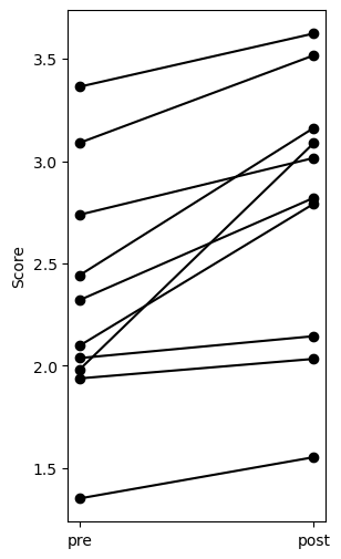
Plot the result:
import matplotlib.pyplot as plt

x = np.zeros_like(agg.values).T + [[0], [1]]
y = agg.values.T

plt.figure(figsize=(3, 6))
plt.plot(x, y, 'o-k')
plt.xticks([0, 1], labels=agg.columns)
plt.ylabel('Score')
plt.show()
Example: Connectomics#
The connectome of the (female) fly brain was recently published.
It can be accessed usign a beautiful web interface and user friendly web site: https://codex.flywire.ai.
The web site is great for exploring the fly brain, but clicking around in a web browser has limitations in terms of the reproducibility and scale of an analysis.
Therefore, the data was made availabel as a set of tables that can be loaded and processed with pandas.
In the exercise, we will use pandas to answer neuroscience questions about the fly brain - here is a brief introduction to the data:
There are three main tables:
connections - connections between cells
classification - cell classes (afferent, intrinsic, efferent), …
(labels - human annotations of cell types)
Each neuron has a unique identifier, the root_id. The root_id can be used to track neurons across the different tables. For instance, to find all neurons of a specific types, and then find their inputs or outputs.
Classifications and connections#
The classification table has basic information about each of the 130k neurons in the fly brain: the cell_type, side of the brain, position in the brain etc.
classification = pd.read_csv('dat/flywire/classification.csv.gz')
classification
| root_id | flow | super_class | class | sub_class | cell_type | hemibrain_type | hemilineage | side | nerve | |
|---|---|---|---|---|---|---|---|---|---|---|
| 0 | 720575940627005443 | intrinsic | optic | L1-5 | NaN | L4 | NaN | NaN | right | NaN |
| 1 | 720575940615995398 | intrinsic | optic | L1-5 | NaN | L4 | NaN | NaN | right | NaN |
| 2 | 720575940621762567 | afferent | ascending | AN | NaN | NaN | NaN | NaN | right | CV |
| 3 | 720575940624384007 | afferent | sensory | olfactory | NaN | NaN | ORN_VA1v | NaN | left | AN |
| 4 | 720575940614422540 | intrinsic | central | NaN | NaN | NaN | AOTU032,AOTU034 | LALa1_posterior | right | NaN |
| ... | ... | ... | ... | ... | ... | ... | ... | ... | ... | ... |
| 127974 | 720575940621500404 | intrinsic | visual_projection | NaN | NaN | NaN | LLPC1,LLPC2a,LLPC2b,LLPC2c,LLPC2d,LLPC3 | NaN | right | NaN |
| 127975 | 720575940651646966 | intrinsic | central | NaN | NaN | NaN | NaN | LB0_anterior | center | NaN |
| 127976 | 720575940630151162 | intrinsic | optic | optic_lobes | NaN | NaN | NaN | NaN | left | NaN |
| 127977 | 720575940629364731 | intrinsic | optic | optic_lobes | NaN | NaN | NaN | NaN | right | NaN |
| 127978 | 720575940623859711 | afferent | sensory | visual | NaN | R1-6 | NaN | NaN | right | NaN |
127979 rows × 10 columns
The connections table contains information about all ~4M synaptic synaptic connections:
pre_root_id: root_id of the presynaptic neuron, the source
post_root_id: root_id of the postsynaptic neuron, the target
syn_count: number of synapses in connection
nt_type: predicted neurotransmitter neurotransmitter
neuropil: target neuropil
connections = pd.read_csv('dat/flywire/connections.csv.gz')
connections
| pre_root_id | post_root_id | neuropil | syn_count | nt_type | |
|---|---|---|---|---|---|
| 0 | 720575940596125868 | 720575940608552405 | LOP_R | 5 | ACH |
| 1 | 720575940596125868 | 720575940611348834 | LOP_R | 7 | ACH |
| 2 | 720575940596125868 | 720575940613059993 | LOP_R | 5 | GLUT |
| 3 | 720575940596125868 | 720575940616986553 | LOP_R | 5 | ACH |
| 4 | 720575940596125868 | 720575940620124326 | LOP_R | 8 | ACH |
| ... | ... | ... | ... | ... | ... |
| 3794610 | 720575940660868737 | 720575940607206786 | ME_L | 9 | GABA |
| 3794611 | 720575940660868737 | 720575940608664873 | ME_L | 6 | GABA |
| 3794612 | 720575940660868737 | 720575940611462242 | ME_L | 6 | GABA |
| 3794613 | 720575940660868737 | 720575940622913063 | ME_L | 23 | GABA |
| 3794614 | 720575940660868737 | 720575940626553546 | ME_L | 6 | ACH |
3794615 rows × 5 columns
Example: Find neurons of a specific cell type#
LC10a is a cluster of higher-order visual neurons required by Drosophila males to track the female during courtship.
We can find all LC10a neurons in the fly brain using boolean indexing into the classification table:
LC10a_neurons = classification[classification['cell_type']=='LC10a']
LC10a_neurons
| root_id | flow | super_class | class | sub_class | cell_type | hemibrain_type | hemilineage | side | nerve | |
|---|---|---|---|---|---|---|---|---|---|---|
| 3035 | 720575940620720112 | intrinsic | visual_projection | NaN | NaN | LC10a | LC10 | VPNd2 | right | NaN |
| 3691 | 720575940638285109 | intrinsic | visual_projection | NaN | NaN | LC10a | LC10 | VPNd2 | left | NaN |
| 3737 | 720575940614430111 | intrinsic | visual_projection | NaN | NaN | LC10a | LC10 | VPNd2 | right | NaN |
| 4456 | 720575940623082237 | intrinsic | visual_projection | NaN | NaN | LC10a | LC10 | VPNd2 | right | NaN |
| 4544 | 720575940623868853 | intrinsic | visual_projection | NaN | NaN | LC10a | LC10 | VPNd2 | left | NaN |
| ... | ... | ... | ... | ... | ... | ... | ... | ... | ... | ... |
| 125773 | 720575940631195217 | intrinsic | visual_projection | NaN | NaN | LC10a | LC10 | VPNd2 | left | NaN |
| 126409 | 720575940631982929 | intrinsic | visual_projection | NaN | NaN | LC10a | LC10 | VPNd2 | left | NaN |
| 126528 | 720575940631983185 | intrinsic | visual_projection | NaN | NaN | LC10a | LC10 | VPNd2 | left | NaN |
| 126843 | 720575940627265223 | intrinsic | visual_projection | NaN | NaN | LC10a | LC10 | VPNd2 | left | NaN |
| 127467 | 720575940610227162 | intrinsic | visual_projection | NaN | NaN | LC10a | LC10 | VPNd2 | left | NaN |
227 rows × 10 columns
Example: Find all postsynaptic partners of a given neuron#
# select the first LC10a neuron in the list and get it's root_id
pre_root_id = LC10a_neurons.iloc[0]['root_id']
print(pre_root_id)

# find all downstream targets for that neuron
# that is, all synaptic connections for which our neuron's root_id is the root_id of the pre-synapse
targets = connections[connections['pre_root_id']==pre_root_id]
targets
720575940620720112
| pre_root_id | post_root_id | neuropil | syn_count | nt_type | |
|---|---|---|---|---|---|
| 1309977 | 720575940620720112 | 720575940610389873 | AOTU_R | 10 | ACH |
| 1309978 | 720575940620720112 | 720575940613946783 | AOTU_R | 10 | ACH |
| 1309979 | 720575940620720112 | 720575940614041238 | AOTU_R | 9 | ACH |
| 1309980 | 720575940620720112 | 720575940616012061 | AOTU_R | 26 | ACH |
| 1309981 | 720575940620720112 | 720575940616169629 | AOTU_R | 14 | ACH |
| 1309982 | 720575940620720112 | 720575940616888020 | AOTU_R | 7 | ACH |
| 1309983 | 720575940620720112 | 720575940619453861 | AOTU_R | 5 | ACH |
| 1309984 | 720575940620720112 | 720575940620321158 | AOTU_R | 11 | ACH |
| 1309985 | 720575940620720112 | 720575940621925631 | AOTU_R | 7 | ACH |
| 1309986 | 720575940620720112 | 720575940622538520 | AOTU_R | 24 | ACH |
| 1309987 | 720575940620720112 | 720575940623107509 | AOTU_R | 5 | ACH |
| 1309988 | 720575940620720112 | 720575940626024336 | AOTU_R | 5 | ACH |
| 1309989 | 720575940620720112 | 720575940626643658 | AOTU_R | 6 | ACH |
| 1309990 | 720575940620720112 | 720575940627738640 | AOTU_R | 22 | ACH |
| 1309991 | 720575940620720112 | 720575940628916444 | AOTU_R | 13 | ACH |
| 1309992 | 720575940620720112 | 720575940628972538 | AOTU_R | 8 | ACH |
| 1309993 | 720575940620720112 | 720575940629883971 | AOTU_R | 17 | ACH |
| 1309994 | 720575940620720112 | 720575940631517251 | AOTU_R | 31 | ACH |
| 1309995 | 720575940620720112 | 720575940638668659 | AOTU_R | 11 | ACH |
| 1309996 | 720575940620720112 | 720575940652922529 | AOTU_R | 11 | ACH |