Numpy#
Exercise 1: Creating arrays#
Create different numpy arrays with the following properties. Use the numpy functions, no for loops!
4-element vector of zeros
2x3 matrix of ones
a sequence of increasing numbers with first element 0, last element 4, interval 0.5
a sequence of 31 numbers with the first element 0 and the last element 4.
# your solution here
Exercise 2: Looping through numpy arrays#
Use a for loop to:
Print each of the 5 rows of the matrix
Print each of the 4 columns of the matrix
Print each of the 20 values in the matrix individually
import numpy as np

a = np.arange(1, 5)
b = np.arange(10, 60, 10)

matrix = a + b[:, np.newaxis]
print(matrix)

# your solution here
[[11 12 13 14]
 [21 22 23 24]
 [31 32 33 34]
 [41 42 43 44]
 [51 52 53 54]]
Exercise 3: Math with arrays#
When creating time values for plotting before we needed lists and for loops:
import matplotlib.pyplot as plt
# say we have 10 data points, sampled every 0.1 seconds, starting at 0 seconds:
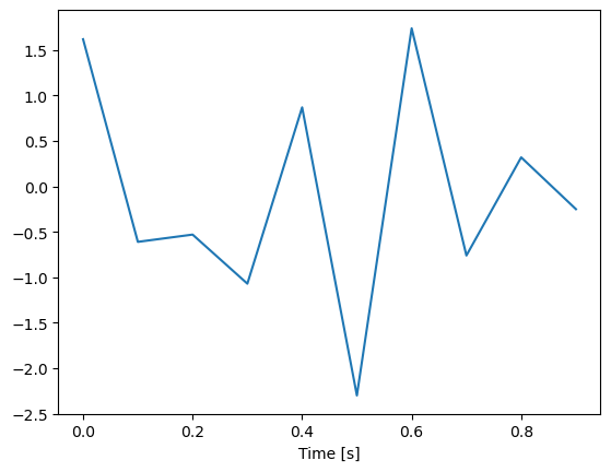
data = [1.62, -0.61, -0.53, -1.07, 0.87, -2.30, 1.74, -0.76, 0.32, -0.25]
step_size = 0.1 # seconds - we want a time axis for the data in seconds
time_seconds = []
for index in range(len(data)):
time_seconds.append(index * step_size)
print(time_seconds)
plt.plot(time_seconds, data)
plt.xlabel('Time [s]')
# DO NOT CHANGE THIS CODE
[0.0, 0.1, 0.2, 0.30000000000000004, 0.4, 0.5, 0.6000000000000001, 0.7000000000000001, 0.8, 0.9]
Text(0.5, 0, 'Time [s]')
Let’s do this using numpy now - without any for loops.
Exercise 3a - time axis starting at 0 seconds#
Our data has 10 values, sampled at an interval of 100 milliseconds, starting at 0 seconds. Use np.arange function to create the array with time value for plotting in a single line. Plot the data and add proper x-axis labels.
# your solution here
Exercise 3b - time axis starting at 2 seconds#
We just realized that we made a mistake - the data were sampled starting at 2 seconds, not at 0 seconds. Add 2 to each value of the time array and replot the data with the new time axis
# your solution here
Exercise 4: Z-scoring our data#
In a previous exercise, we have z-scored some temperature data using core python and a bunch of for loops.
Remember that z-scoring amounts to for each value: subtracting the mean, \(M\), and dividing by the standard deviation, \(S\): \(z_i = (x_i - M) / S\)
# EXECUTE BUT DO NOT CHANGE THIS CELL
temperature_anomalies = [-0.19,-0.177,-0.308,-0.289,-0.193,-0.057,0.077,0.026,0.029,0.068,0.256, 0.342, 0.591, 0.792]
print(temperature_anomalies)

# compute mean
mean = 0
for ta in temperature_anomalies:
    mean = mean + ta
mean = mean / len(temperature_anomalies)

# compute std
std = 0
for ta in temperature_anomalies:
    std = std + (ta - mean) ** 2
std = (std / len(temperature_anomalies)) ** (1/2)

# z-score - subtract the mean and divide by the standard deviation
ta_zscored = []
for ta in temperature_anomalies:
    ta_zscored.append( (ta - mean) / std)

ta_zscored
[-0.19, -0.177, -0.308, -0.289, -0.193, -0.057, 0.077, 0.026, 0.029, 0.068, 0.256, 0.342, 0.591, 0.792]
[-0.8220097542568958,
 -0.7807619529680193,
 -1.1964128736482362,
 -1.1361276256106474,
 -0.8315284776312519,
 -0.4000130179937748,
 0.025156626060798284,
 -0.13666167130325566,
 -0.12714294792889955,
 -0.0033995440622700372,
 0.5931071207307131,
 0.8659771907955884,
 1.6560312308671457,
 2.2937856969490054]
This is quite a bit of code. Use Numpy to get z-score the data in 1-2 lines of code, without any for loops. You can use np.mean and np.std to compute the mean and standard deviation
# EXECUTE BUT DO NOT CHANGE THIS CELL
temperature_anomalies = [-0.19,-0.177,-0.308,-0.289,-0.193,-0.057,0.077,0.026,0.029,0.068,0.256, 0.342, 0.591, 0.792]
print(temperature_anomalies)

# your solution here
[-0.19, -0.177, -0.308, -0.289, -0.193, -0.057, 0.077, 0.026, 0.029, 0.068, 0.256, 0.342, 0.591, 0.792]
Exercise 5: Slice indexing#
You are given a matrix. Use slice indexing to:
print the second row
print the 6th column
print every second column
print the upper left 3x3 matrix
print the lower right 2x2 matrix
print the matrix with out the first and last row and first and last column
set the lower left 3x3 matrix to 0
import numpy as np

matrix = np.arange(10)[:, np.newaxis] + np.arange(10)[np.newaxis, :]
print(matrix)

# your solution
[[ 0  1  2  3  4  5  6  7  8  9]
 [ 1  2  3  4  5  6  7  8  9 10]
 [ 2  3  4  5  6  7  8  9 10 11]
 [ 3  4  5  6  7  8  9 10 11 12]
 [ 4  5  6  7  8  9 10 11 12 13]
 [ 5  6  7  8  9 10 11 12 13 14]
 [ 6  7  8  9 10 11 12 13 14 15]
 [ 7  8  9 10 11 12 13 14 15 16]
 [ 8  9 10 11 12 13 14 15 16 17]
 [ 9 10 11 12 13 14 15 16 17 18]]
Exercise 6 - Boolean indexing#
We are given a numpy array, x of data values.
No for loops allowed in this exercise!
Exercise 6a - comparisons on arrays in numpy#
Using numpy (no for loops) and comparison operators, generate an new boolean array greater_zero that has the value True at all indices for which x is >0, and False otherwise:
import numpy as np
x = np.array([0.154, -0.135, -1.362, -0.658, 1.908, -1.152, 0.381, -1.258, 0.436, -0.667, -0.936, 0.601, 0.483, 0.567, 1.277, 0.965, -0.321, -1.43, -0.367, -0.925, -0.067, 1.121, -0.313, 0.36, 0.48, 0.401, 0.659, 0.461, 0.652, 1.053])

# your solution here
Exercise 6b - boolean indexing (1)#
Expand on your solution above. Use boolean indexing to print
all values >0
all values <0
import numpy as np
x = np.array([0.154, -0.135, -1.362, -0.658, 1.908, -1.152, 0.381, -1.258, 0.436, -0.667, -0.936, 0.601, 0.483, 0.567, 1.277, 0.965, -0.321, -1.43, -0.367, -0.925, -0.067, 1.121, -0.313, 0.36, 0.48, 0.401, 0.659, 0.461, 0.652, 1.053])

# your solution here
Exercise 6c - boolean indexing (2)#
Expand again on your solution to compute the mean of:
all values >0
all values <0
import numpy as np
x = np.array([0.154, -0.135, -1.362, -0.658, 1.908, -1.152, 0.381, -1.258, 0.436, -0.667, -0.936, 0.601, 0.483, 0.567, 1.277, 0.965, -0.321, -1.43, -0.367, -0.925, -0.067, 1.121, -0.313, 0.36, 0.48, 0.401, 0.659, 0.461, 0.652, 1.053])

# your solution here
Exercise 7: Searching arrays#
Exercise 7a - counting True values (Important)#
In the array x, how many values:
are <0
are >0
are >-0.5 and <0.5
Do not use a for loop. Use boolean indexing!
import numpy as np
x = np.array([0.154, -0.135, -1.362, -0.658, 1.908, -1.152, 0.381, -1.258, 0.436, -0.667, -0.936, 0.601, 0.483, 0.567, 1.277, 0.965, -0.321, -1.43, -0.367, -0.925, -0.067, 1.121, -0.313, 0.36, 0.48, 0.401, 0.659, 0.461, 0.652, 1.053])

# your solution here
Exercise 7b - getting the indices of True values#
Given the following array of data values, use np.where to get the indices at which:
the data is <0
the data is >0
Do not use a for loop. Use boolean indexing!
import numpy as np
x = np.array([0.154, -0.135, -1.362, -0.658, 1.908, -1.152, 0.381, -1.258, 0.436, -0.667, -0.936, 0.601, 0.483, 0.567, 1.277, 0.965, -0.321, -1.43, -0.367, -0.925, -0.067, 1.121, -0.313, 0.36, 0.48, 0.401, 0.659, 0.461, 0.652, 1.053])

# your solution here
Exercise 8: Spike detection#
Let’s implement the simple spike detection task using numpy.
Download the file “voltage_trace.npz” from the files section on StudIP and put it in the same folder as this notebook.
Load the data by executing the cell below.
# RUN THIS CELL TO LOAD THE DATA
import numpy as np

data = np.load('voltage_trace.npz')
times = data['times_seconds']
voltages = data['voltage_trace']
# RUN THIS CELL TO LOAD THE DATA
Exercise 8b: Detect spikes using numpy#
This is our spike detection code, using core python:
threshold = 10
spike_times_old = []
spike_voltages_old = []

for index in range(len(voltages)):
    v = voltages[index]
    t = times[index]
    if v > threshold:
        spike_voltages_old.append(v)
        spike_times_old.append(t)
print(f"Detected {len(spike_times_old)} spikes.")
Detected 61 spikes.
Turn this into numpy code. Do not use a for-loop. Use boolean indexing.
# your solution here
Exercise 8c: Plot the voltage trace and overlay the spike times generated by both methods#
The spikes detected using the old python code should be marked as vertical red lines (use plt.axvline), the spikes detected using numpy should be marked as green dots at their peaks. Like so:

Did you catch every spike?
# your solution here
Exercise 9: Chunking (bonus)#
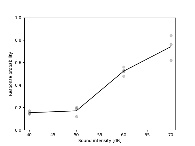
We ran an experiment in which we trained a rat to detect a short tone pip. We now tested the rat’s detection performance by presenting the tone pip at different intensities and calculating the detection probability. Load and plot the raw data and compute and plot the mean response probabiltity for each intensity.
Download the file “sound_expt.xlsx” from the Files section on studip, load it and cast it to a numpy array (ask the internet if you do not know how to load excel files and cast them to numpy). In parallel, open the data file in excel to determine how the data is structured (which columns hold which information)
Compute the mean of the response probability values for each sound intensity value.
Plot the individual data points and overlay a curve with the mean responses probability per sound intensity. Roughly like so:
Exercise 9a: Load the data with pandas and cast it to numpy#
# your solution here
Exercise 9b: Compute the mean over stimulus response probabilities obtained for the same sound intensity#
# your solution here
Exercise 9c: Plot the individual data as points and the mean values as a curve#
The x-axis should be sound intensity, the y-axis response probability.
# your solution here