Bonus exercises: Temperature anomalies#
# EXECUTE BUT DO NOT CHANGE
import numpy as np

def load_anomalies():
    # Load the full anomaly data set
    data = np.loadtxt('temperature.csv', skiprows=1, delimiter=',')
    years = [int(y) for y in data[:, 0]]  # unpack the table and cast years to int
    temperature_anomalies = list(data[:, 1])  # unpack the table
    return years, temperature_anomalies

years, temperature_anomalies = load_anomalies()
print(years[:10])
print(temperature_anomalies[:10])
[1880, 1881, 1882, 1883, 1884, 1885, 1886, 1887, 1888, 1889]
[np.float64(-0.1), np.float64(-0.17), np.float64(-0.11), np.float64(-0.17), np.float64(-0.28), np.float64(-0.26), np.float64(-0.27), np.float64(-0.22), np.float64(-0.09), np.float64(-0.23)]
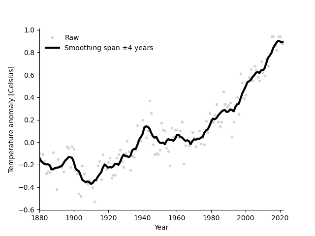
Exercise 1: Smooth the anomaly values#
Smooth using a moving average window spanning +/-4 of the neighbouring values.
To smooth with a span of 4, you replace each data point with the average value of 9 values:
the datapoint itself,
the 4 preceeding, and
the 4 following values.
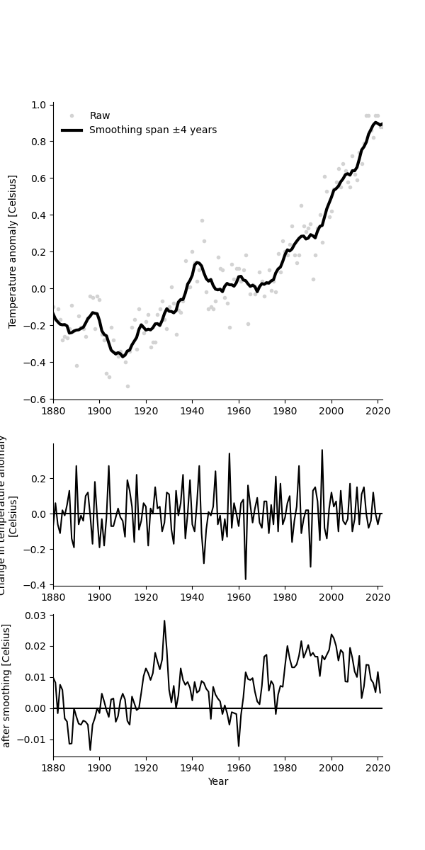
Label and format the plot, and plot the raw values as dots and the smoothed values as a line, as in the figure below.
Roughly like so:
# Your solution here
import matplotlib.pyplot as plt

def mean(values):

    avg = 0
    for value in values:
        avg = avg + value

    avg = avg / len(values)

    return avg

def smooth(data, span=4):
    smoothed = []

    for idx in range(len(data)):
        start = max(0, idx-span)
        end = min(len(data), idx+span+1)

        values = data[start:end]

        avg = mean(values)
        smoothed.append(avg)

    return smoothed

spans = [1, 2, 4, 8, 16]
for span in spans:
    plt.plot(smooth(temperature_anomalies, span=span))
plt.show()
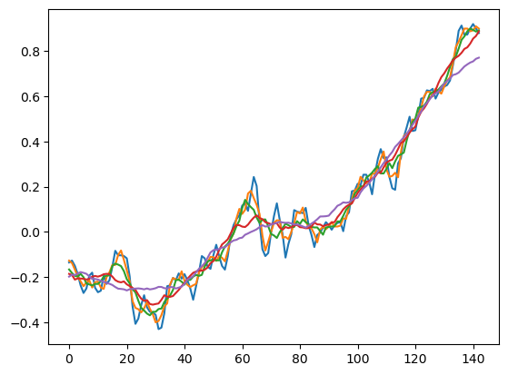
Exercise 2: Make your code more readable by using functions#
Write function that smooths its inputs.
change = []

for idx in range(len(temperature_anomalies) - 1):
    start = idx + 1
    end = idx


    diff = temperature_anomalies[start] - temperature_anomalies[end]
    change.append(diff)

plt.plot(smooth(change, span=8))
plt.axhline(0)
<matplotlib.lines.Line2D at 0x137fd4690>
# Your solution here
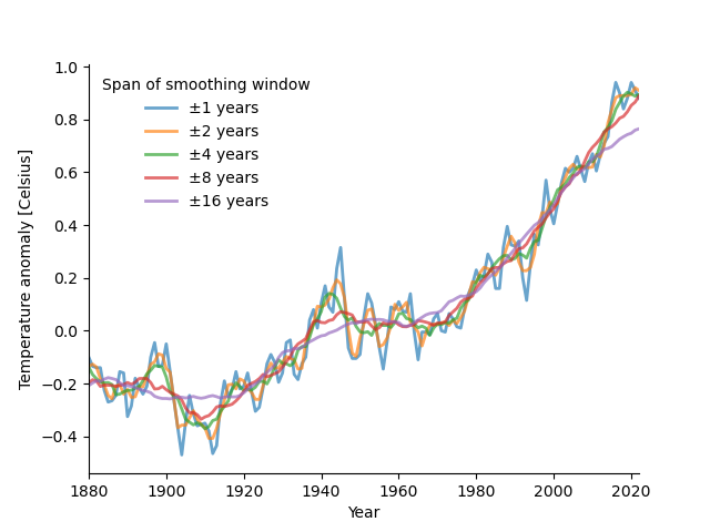
Exercise 3: Smooth the anomaly values with different spans#
Use different spans of the moving average window (1, 2, 4, 8, 16). Overlay smoothed values for the different spans. Make a function for smoothing to simplify your code.
The plot should look roughly like so:
# your solution
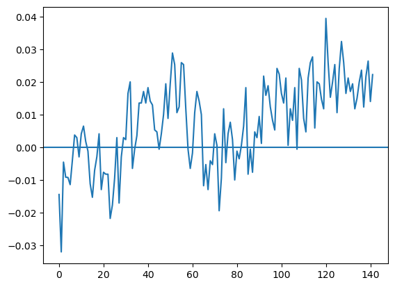
Exercise 4: Change in temperature anomalies#
Plot the year-over-year change in anomaly values.
Smooth the change using a moving average window spanning +/-2 neighbouring values.
Compute the difference between the smoothed and the raw values.
Plot the raw change as dots and the smoothed change as lines.
Roughly like so:
# your solution