Probabilities#
You tested a new wonder drug that is supposed to increase to score of mice in a learning assay.
The test scores from a group of control and of treatment animals are stored in a file.
Explore the data using histograms and descriptive statistics.
Exercise 1: Load the data and determine sample sizes#
Download the file 5.01_probabilities_exercise.npz from studip.
Load and inspect the data.
What are the sample sizes for the control and treatment data?
# your solution here
Exercise 2: Visualize the probability densities#
Plot the probability densities for the control and treatment data. Plot them in the same plot so you can directly compare them.
Hint: To make the overlapping histograms more easily visible, make them translucent by setting the alpha argument to 0.5. Something like plt.hist(x, bins=1_000, alpha=0.5).
# your solution here
Exercise 3: Calculate mean, standard deviation, and standard error of the mean for both distributions#
Calculate and compare the standard deviation (std) and the standard error of the mean (sem) for both data sets.
Can you explain why the std is higher for the treatment data, but the sem is lower for the control data?
HINT: If your data is represented as a dictionary, you can use a for loop and .items() to compute the statistics for each key-value pair.
# your solution here
Exercise 4: Plot with different types of errorbars#
Plot the means of control and treatment data with error bars.
Produce two plots with different definitions of the error bars:
standard deviation
standard error of the mean
Roughly like so:
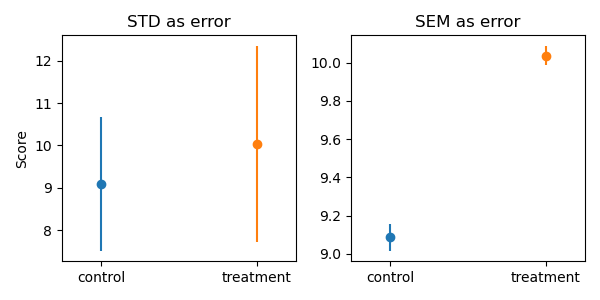
Compare the magnitude of the error bars in the two plots.
# your solution here
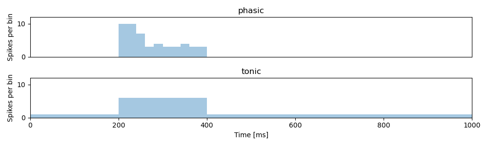
Exercise 5: Visualizing firing rates using a PSTH#
You are give a dictionary with the spike times produced by a phasic and a tonic neuron. Both were stimulated with a current injection between 200-400ms. The total duration of the recording is 1000ms.
Visualize how the firing rate of each neuron changes during the recording using a Peri-Stimulus-Time-Histogram (PSTH). A PSTH is nothing more than a histogram of the spike times!
To compare the PSTHs, use histograms with the same bins for both neurons, starting at 0ms, ending at 1000ms, with a bin size of 20 ms.
Plot the PSTHs for both neurons in subplots, roughly like so:
import numpy as np
spike_times = {'phasic': np.concatenate((np.arange(200, 250, 2), np.arange(250, 400, 6))),
         'tonic': np.concatenate((np.arange(200, 400, 4), np.arange(0, 1000, 20))),
}
print(spike_times)
# your solution here:
{'phasic': array([200, 202, 204, 206, 208, 210, 212, 214, 216, 218, 220, 222, 224,
       226, 228, 230, 232, 234, 236, 238, 240, 242, 244, 246, 248, 250,
       256, 262, 268, 274, 280, 286, 292, 298, 304, 310, 316, 322, 328,
       334, 340, 346, 352, 358, 364, 370, 376, 382, 388, 394]), 'tonic': array([200, 204, 208, 212, 216, 220, 224, 228, 232, 236, 240, 244, 248,
       252, 256, 260, 264, 268, 272, 276, 280, 284, 288, 292, 296, 300,
       304, 308, 312, 316, 320, 324, 328, 332, 336, 340, 344, 348, 352,
       356, 360, 364, 368, 372, 376, 380, 384, 388, 392, 396,   0,  20,
        40,  60,  80, 100, 120, 140, 160, 180, 200, 220, 240, 260, 280,
       300, 320, 340, 360, 380, 400, 420, 440, 460, 480, 500, 520, 540,
       560, 580, 600, 620, 640, 660, 680, 700, 720, 740, 760, 780, 800,
       820, 840, 860, 880, 900, 920, 940, 960, 980])}