Ultrasonic vocalizations from mice

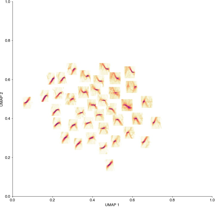
Mouse USVs do not cluster into discrete types but lie on a continuous, low-dimensional manifold.

We here closely follow the procedure described in Sainburg et al. (2020): Finding, visualizing, and quantifying latent structure across (see code on github).

import numpy as np
import matplotlib
import matplotlib.pyplot as plt
import librosa.feature
import colorcet as cc
import umap
import scipy.cluster.vq
import das_unsupervised.spec_utils
from io import BytesIO
import urllib.request

%config InlineBackend.figure_format = 'jpg'  # smaller mem footprint for page
plt.style.use('ncb.mplstyle')

Download audio data

Data kindly provided by Kurt Hammerschmidt and published in A Ivanenko, P Watkins, MAJ van Gerven, K Hammerschmidt, B Englitz (2020) Classifying sex and strain from mouse ultrasonic vocalizations using deep learning. PLoS Comput Biol 16(6): e1007918.

url = 'https://github.com/janclemenslab/das_unsupervised/releases/download/v0.4/mice.npz'
with urllib.request.urlopen(url) as f:
    ff = BytesIO(f.read())

d = np.load(ff)
samplerate = d['samplerate']
recording = d['recording']
syllable_onsets = d['syllable_onsets']
syllable_offsets = d['syllable_offsets']

Pre-processing

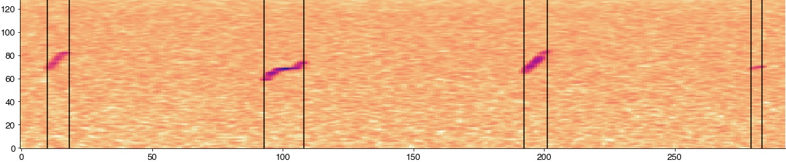
Compute the spectrogram

n_fft = 2048
hop_length = int(samplerate / 1000)

specgram = librosa.feature.melspectrogram(recording, sr=samplerate, n_fft=n_fft, hop_length=hop_length, power=1, fmin=40_000)
freqs = librosa.core.mel_frequencies(n_mels=specgram.shape[0], fmin=40_000, fmax=int(samplerate/2), htk=False)
sm = np.median(specgram, axis=1)
print(sm.shape)

plt.figure(figsize=(20, 4))
plt.imshow(np.log2(specgram[:, int(syllable_onsets[1]/hop_length)-10:int(syllable_offsets[4]/hop_length)+10]), cmap='cet_CET_L17')
for onset, offset in zip(syllable_onsets[1:5], syllable_offsets[1:5]):
    plt.axvline((onset-syllable_onsets[1])/hop_length + 10, c='k')
    plt.axvline((offset-syllable_onsets[1])/hop_length + 10, c='k')
plt.show()

(128,)

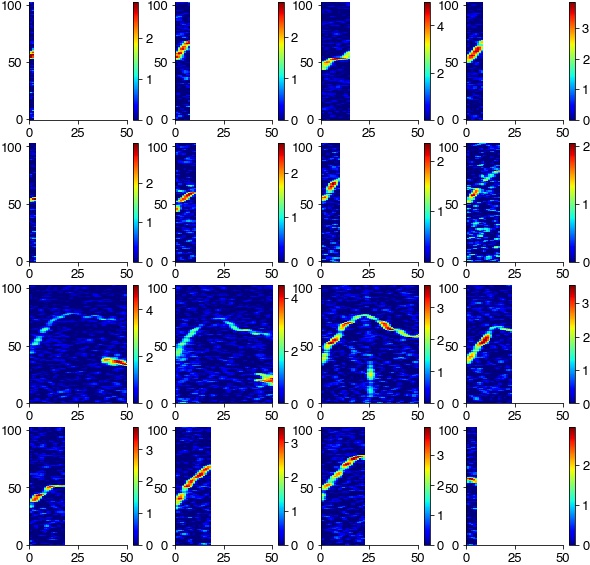
Extract and threshold syllables from spectrogram

specs = [] 

plt.figure(figsize=(10, 10))
for cnt, (onset, offset) in enumerate(zip(syllable_onsets, syllable_offsets)):
    spec = np.log2(specgram[:, int(onset/hop_length):int(offset/hop_length)]/ sm[:,np.newaxis])
    spec = spec[15:-10, :]
    spec[spec<0] = 0
    specs.append(spec)
    try:
        plt.subplot(4,4,cnt+1)
        plt.imshow(spec, cmap='jet')
        plt.xlim(0, 50)
        plt.colorbar()
    except:
        pass

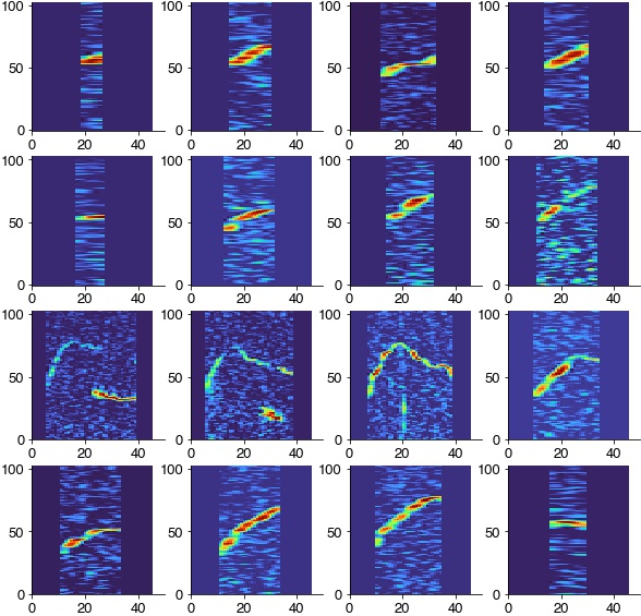
Log-scale the time axis to reduce differences in syllable duration and zero-pad all syllables to the same duration

spec_rs = [das_unsupervised.spec_utils.log_resize_spec(spec, scaling_factor=8) for spec in specs]

max_len = np.max([spec.shape[1] for spec in spec_rs])
print(max_len)
spec_rs = [das_unsupervised.spec_utils.pad_spec(spec, pad_length=max_len) for spec in spec_rs]
plt.figure(figsize=(10, 10))
for cnt, spc in enumerate(spec_rs[:16]):
    plt.subplot(4,4,cnt+1)
    plt.imshow(spc, cmap='turbo')
    plt.xlim(0, 50)

46

Center spectra around their peak frequencies

offset = 20
spec_rs_c = [das_unsupervised.spec_utils.center_spec(spec, halfwidth=offset) for spec in spec_rs]
spec_rs_c = np.array(spec_rs_c)

Flatten 2D [time x freq] spectrograms to 1D feature vectors

spec_flat = [spec.ravel() for spec in spec_rs_c]
spec_flat = np.array(spec_flat)

Dimensionality reduction and clustering

Embed the feature vectors into a 2D space using UMAP and group similar syllables usign kmeans.

out = umap.UMAP(min_dist=0.5, random_state=2).fit_transform(spec_flat)
k_centroid, k_labels = scipy.cluster.vq.kmeans2(out, k=40, seed=2)

/Users/clemens10/miniconda3/lib/python3.7/site-packages/scipy/cluster/vq.py:607: UserWarning: One of the clusters is empty. Re-run kmeans with a different initialization.
  warnings.warn("One of the clusters is empty. "

Plot results

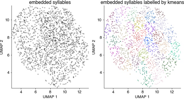
Syllable spectrograms embedded into a 2D space (left) and colored by the unsupervised cluster labels (right). Syllables do not fall into separate groups, but can be grouped by similarity using clustering.

plt.figure(figsize=(10, 5))

plt.subplot(121)
plt.scatter(out[:,0], out[:,1], c='k', alpha=0.25, s=8)
plt.axis('tight')
plt.xlabel('UMAP 1')
plt.ylabel('UMAP 2')
plt.title('embedded syllables')

plt.subplot(122)
plt.scatter(out[:,0], out[:,1], c=k_labels, cmap='cet_glasbey_dark', alpha=0.5, s=8, edgecolor='none')
plt.axis('tight')
plt.xlabel('UMAP 1')
plt.ylabel('UMAP 2')
plt.title('embedded syllables labelled by kmeans')

plt.show()

Average spectrograms of the syllables in each cluster, plotted at the position of the respective cluster centroid in UMAP space. Spectrotemporal features vary smoothly within this space, suggesting that mouse USVs lie on a low-dimensional manifold.

fig = plt.figure(figsize=(12, 12))
ax = plt.axes()
for cnt, (centroid, label) in enumerate(zip(k_centroid, np.unique(k_labels))):
    idx = np.where(k_labels==label)[0]
    X = np.mean(spec_rs_c[idx], axis=0)
    fig.figimage(X=X, xo=centroid[0]*40, yo=centroid[1]*40, cmap='cet_CET_L17')
plt.xlabel('UMAP 1')
plt.ylabel('UMAP 2')
plt.show()